Bayer patterned high dynamic range image reconstruction using adaptive weighting function

R E S E A R C H

Open Access

Bayer patterned high dynamic range image

reconstruction using adaptive weighting

function

Hee Kang

, Suk Ho Lee

, Ki Sun Song

and Moon Gi Kang

Abstract

It is not easy to acquire a desired high dynamic range (HDR) image directly from a camera due to the limited dynamic range of most image sensors. Therefore, generally, a post-process called HDR image reconstruction is used, which reconstructs an HDR image from a set of differently exposed images to overcome the limited dynamic range.

However, conventional HDR image reconstruction methods suffer from noise factors and ghost artifacts. This is due to the fact that the input images taken with a short exposure time contain much noise in the dark regions, which contributes to increased noise in the corresponding dark regions of the reconstructed HDR image. Furthermore, since input images are acquired at different times, the images contain different motion information, which results in ghost artifacts. In this paper, we propose an HDR image reconstruction method which reduces the impact of the noise factors and prevents ghost artifacts. To reduce the influence of the noise factors, the weighting function, which determines the contribution of a certain input image to the reconstructed HDR image, is designed to adapt to the exposure time and local motions. Furthermore, the weighting function is designed to exclude ghosting regions by considering the differences of the luminance and the chrominance values between several input images. Unlike conventional methods, which generally work on a color image processed by the image processing module (IPM), the proposed method works directly on the Bayer raw image. This allows for a linear camera response function and also improves the efficiency in hardware implementation. Experimental results show that the proposed method can reconstruct high-quality Bayer patterned HDR images while being robust against ghost artifacts and noise factors.

Keywords: High dynamic range; Bayer pattern; Camera response function; Ghost artifact

1 Introduction

Image capturing devices like digital cameras and cam-corders have recently improved remarkably. However, image sensors such as charge-coupled devices (CCD) and complementary metal-oxide semiconductors (CMOS) in these imaging devices can still only capture a limited dynamic range. As a result, when a captured scene con-tains a dynamic range above the given limitation, a loss of information is inevitable even if the exposure is adjusted according to the brightness of the scene. Thus, many methods based on signal processing have been proposed to reproduce scenes with a high dynamic range (HDR).

*Correspondence: [email protected]

1Department of Electric and Electronic Engineering, Yonsei University, 50 Yonsei-ro, Seodaemun-gu, Seoul 120-749, Korea

Full list of author information is available at the end of the article

To obtain HDR images, many HDR imaging approaches utilize low dynamic range (LDR) images with different exposures [1-11]. Most of these approaches first convert the pixel values of input images into radiance values by using the camera response function (CRF), where the CRF refers to the function that maps the radiance values of a given scene to the pixel values in the captured image, and the radiance refers to the physical quantity of light energy on each element on the sensor array. Next, the radiance values of the input images are combined into a single HDR image using weighting functions based on the reliability of the input data.

In early studies, conventional approaches were pro-posed to estimate the CRF from multiple LDR images. These CRF estimation approaches can be categorized as parametric [1,2] and non-parametric approaches [3,4]. In parametric approaches, Mann and Picard [1] presented a

variety of parametric forms for CRF estimation. Mitsunaga and Nayar [2] used a high-order polynomial function to estimate the CRF. On the other hand, in terms of non-parametric approaches, Debevec and Malik [3] estimated the CRF using an objective function with a smoothness constraint. Pal et al. [4] used a Bayesian network consist-ing of a probabilistic model for an imagconsist-ing function and a generative model for smooth functions.

In recent years, some techniques have been proposed to prevent artifacts in HDR images caused by moving objects [5-10]. If local motion occurs in a scene while the LDR images are being captured, a ghost artifact appears in the HDR image. Most of the ghost artifact-preventing tech-niques first detect the local motion by using ghost artifact measurement and then combine the LDR images without the ghost artifact regions.

All these approaches, however, combine LDR images without considering the influence of noise factors. Dark regions in an LDR image taken with short exposure time contain relatively more noise factors because the regions are under-exposed or noisy. Thus, the noise level is increased in the corresponding dark regions of the recon-structed HDR image. These approaches also utilize RGB images processed by the image processing module (IPM). The IPM is a processor which converts Bayer raw data into an RGB image suitable to the human visual system [12-14]. Using RGB images processed by the IPM makes the CRF estimation inaccurate since the IPM includes sev-eral adaptive nonlinear sub-modules, e.g., dynamic range compression, noise reduction [15], and color correction [16] algorithms. An inaccurate CRF leads to poor HDR imaging performance. Moreover, the use of RGB images increases the hardware complexity since the IPM has to be performed several times before the HDR image recon-struction, as shown in Figure 1a.

In this paper, we introduce a new approach which per-forms HDR image reconstruction on the Bayer raw images before the IPM [17], as shown in Figure 1b. The pro-posed method can be widely used in applications such as real-time HDR video cameras because of the reduction of hardware complexity. The CRF estimation is simpler and more accurate than conventional methods because the CRF before the IPM is linear. The proposed method considers the noise and the ghost artifact problems. For this purpose, a new weighting function is proposed to combine the Bayer patterned LDR (BP-LDR) images. The proposed weighting function is designed so that each of the BP-LDR images independently covers each corre-sponding region according to the radiance value in order to reduce the influence of the noise. The regions covered by each BP-LDR image are determined by the exposure of each BP-LDR image and the existence of local motion. This avoids using the short-exposure BP-LDR image to reconstruct the dark regions in the Bayer patterned HDR

(BP-HDR) image. The weighting function also detects the local motion in the Bayer pattern and excludes ghosting regions. To detect the local motion, the luminance and the chrominance values are directly calculated in the Bayer pattern, and the differences of these values are utilized. When the proposed method is compared with conven-tional methods, the detection performance is improved since an accurate CRF is employed.

The rest of this paper is organized as follows: In Section 2, the proposed BP-HDR image reconstruction approach is described in detail. The properties of the CRF are discussed and analyzed in Section 2.1. Section 2.2 describes the design process of the adaptive weighting function for BP-HDR image reconstruction. In Section 3, experimental results of various test images are presented, and the paper is concluded in Section 4.

2 Proposed BP-HDR image reconstruction

2.1 Properties of the camera response function

In general, the radiance valueIRwhich passes through the lens of the camera is converted into a pixel valueIby the image sensor and the IPM part. The CRF is a function that relates the radiance value to the pixel value and is expressed as

I=fIR·t (1)

wheretrepresents the exposure time.

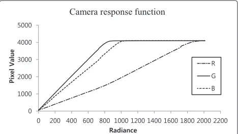
CCD and CMOS image sensors are widely used in image acquisition systems. Both of these sensors utilize the same kind of element called photodiode [18], which generates a current proportional to the light energy. The photodi-ode offers a high level of resistance when there is no light falling on it. On the other hand, the resistance of the pho-todiode is reduced and the current increases linearly with the light energy when light falls on it. That is, the response function of the photodiode is linear with respect to the radiance value. An example under the condition with 6500 k fluorescent lighting using a CMOS sensor with Bayer pattern is shown in Figure 2. In the plot of the pixel value versus the intensity of the radiance, each of these response functions appear to be linear.

(a)

HDR image reconstruction

IPM

IPM

IPM

Conventional methods

Bayer patterned LDR images

RGB LDR images

RGB HDR image

(b)

HDR image

reconstruction

IPM

Proposed method Bayer pattern

Bayer patterned LDR images

Bayer patterned HDR image

RGB HDR image

Figure 1Comparison of hardware complexity when using (a) conventional methods and (b) the proposed method.

the CRF before the IPM and apply it to the BP-LDR images to reconstruct the BP-HDR image.

In the BP-LDR images, the CRF is expressed linearly as f(x) = αx+βas shown in Figure 2. Here,α represents the slope of the CRF corresponding to the sensitivity of the RGB channels. That is,αdiffers according to the color

Camera response function

Figure 2Camera response function of the RGB channels in the Bayer raw data.

channel of the Bayer pattern. However, there is no need to estimateαbecause the auto white balance sub-module of IPM adjusts the slopes of the RGB channels to be equal [14]. Therefore,f(·)can be approximated asf(x)=x+β. β represents the black level of an image sensor which can be simply estimated as the average of the optical black region located on the boundary of the image sensor [21].

2.2 Proposed design method of the weighting function for BP-HDR image reconstruction

the reconstruction process. The reconstructed BP-HDR

whereWnrepresents the weighting function correspond-ing to then-th BP-LDR image,In(i,j)represents the given pixel value at the positioni,jof then-th BP-LDR image, tn represents the exposure time of In, and N is the number of BP-LDR images. For convenience, we arranged I1,I2,. . ..,In,. . .,IN such thatt1> t2> . . ..> tn > . . ..> tN. Furthermore,f represents the CRF explained in the previous section, and thusf−1(In) /tnrepresents the radiance value of In. Therefore, (2) can be regarded as an equation which combines the radiance values of the BP-LDR into the BP-HDR image.

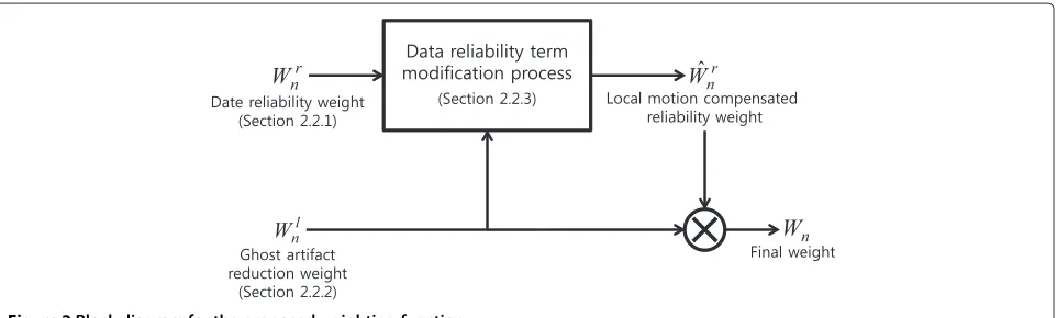
Figure 3 shows a block diagram of the proposed method regarding the estimation of the proposed weighting func-tion. In order to estimate the weighting functionWn, first, the weight for the data reliability (W_nr) and the weight for the ghost artifact reduction (W_nl) have to be estimated. The data reliability weightW_nr is further modified toWˆ_nr to reflect the change of the data reliability according to the ghosting regions in the other LDR images. Then, finally,

ˆ

Wr

n andWnl are combined to obtain the final weighting functionWn:

Wn(i,j)= ˆW_nr(i,j)·W_nl(i,j), (3) The details are described in the following sections.

2.2.1 The weight for data reliability

Conventional methods use a symmetric weighting func-tion that decreases with the distance from the center of the pixel value range [3,11]. This is based on the fact that the pixel values near the center are the most reli-able. If considering only the influence of the noise, the higher part of the pixel value range seems to be reli-able since the shot noise in general image sensor has a Poisson distribution. However, since the higher part is close to the saturation value and since post-processing methods such as the gamma correction make the higher part more close to the saturation value, a smaller weight should be assigned to the higher part to prevent the use of the saturated pixel values in the reconstruction pro-cess. Figure 4a shows two examples of weighting functions that are generally used. These weighting functions are converted into the functions in the radiance domain, as shown in Figure 4b. Using the function values in the radi-ance domain, the ratio of how much the BP-LDR images are combined into the BP-HDR image is calculated. For example, the radiance valueL1in Figure 4b has a weight

of about 0.6 (point a) in the middle exposure BP-LDR image, while the weights in the other BP-LDR images are about 0.2 (point b). This means the weight for the middle

exposure is about three times larger than the weights for the other exposures atL1. In general, it can be observed

that a BP-LDR image captured with long exposure has a large weight in the low-radiance region, while a BP-LDR image captured with short exposure has a large weight in the high-radiance region. However, a major problem is that the short-exposure BP-LDR image has a consid-erable weight in the very low radiance region. Using the short-exposure BP-LDR image in the low-radiance region is improper since it can be under-exposed or noisy in this region.

To overcome the abovementioned problems, we use a designing method for the reliability function. The design-ing method consists of two steps as listed in Algorithm 1. The first step is to design a desired weighting function (W˜_nr) in the radiance domain. The second step is the con-version of the designed weighting function in the radiance domain into that in the pixel value domain.

Algorithm 1 Designing method for the data reliability weighting function

Designing method: Step 1:

Design a desired weighting functionW˜_nr in the radi-ance domain.

Step 2:

Obtain the functionW_nr(·)in the pixel value domain by considering the following relations:

˜

Wr

n(InR)=Wnr(In)andI_nR=f−1(In) /tn.

Thus, the weighting function W_nr(·) is obtained as Wr

n(·)= ˜Wnrf−1(·)/tn.

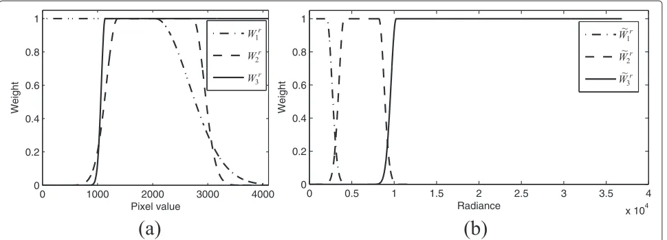
In the first step, the design ofW˜_nrhas to be done so that for a certainn,W˜_nrcovers only a certain region in the radi-ance domain, as shown in Figure 5b. That is, we design the weighting function so that the short-exposure BP-LDR image has an effect only in the high-radiance region, while the long-exposure BP-LDR image has an effect only in the low-radiance region. This reduces the amount of noise in the reconstructed BP-HDR image, since the short-exposure BP-LDR image, which normally contains noise in the dark regions, is not used to reconstruct the low-radiance region in the BP-HDR image.

To make the design simple, the following constraints are used:

1. The two adjacent functionsW˜_nrandW˜_nr₊₁intersect at the same point as in conventional methods. 2. All of the functionsW˜nhave the same slopes at the

transition region.

r n

W

l n

W

W

r n Wˆ

Figure 3Block diagram for the proposed weighting function.

consistent with that in conventional methods. However, since the conventional weighting functions are designed to adapt to the RGB images processed by the image pro-cessing module such as the gamma correction, they are improper for the BP-LDR images. Therefore, we mod-ify the conventional weighting functions to adapt to the BP-LDR images. That is, the maximum value posi-tion (ρ) in the weighting functions is changed from

the center of the pixel value range to a more reliable position as will be later mentioned in Section 3. By obeying the second constraint, the change of the two weights between different exposure LDR images becomes close to linear. This can prevent artifacts which can be possibly generated due to a nonlinear change in the weight ratio. To reduce the overlap between adjacent weighting functions while obeying the above mentioned

0 1000 2000 3000 4000 0

0.2 0.4 0.6 0.8 1

Pixel value

Weight

0 1000 2000 3000 4000 0

0.2 0.4 0.6 0.8 1

Pixel value

Weight

)

b

(

)

a

(

0 0.5 1 1.5 2 2.5 3 3.5 4

x 104 0

0.2 0.4 0.6 0.8 1

Radiance

Weight

0 0.5 1 1.5 2 2.5 3 3.5 4

x 104 0

0.2 0.4 0.6 0.8 1

Radiance

Weight

a

b

c

W1 c

W2 c

W3

c

W1 c

W2 c

W3

)

0 1000 2000 3000 4000 0

Figure 5Proposed weighting function for reliability of the data.(a)In the pixel value domain and(b)in the radiance domain.

constraints, the slopes at the transition region have to be increased.

The proposed weighting functions are calculated start-ing with that correspondstart-ing to the longest exposure image. As shown in Figure 5b,W˜₁r for the longest expo-sure BP-LDR imageI1is asymmetric with respect to point μH

Here,Crepresents the parameter that controls the slope of the functionW˜₁r.

Obeying the second constraint,C should be the same for all ofW˜_nr. ForI₁R < μH₁, W˜₁r has the value 1 sinceI1

is the most reliable in this range. ForI₁R≥μH₁,W˜₁r is the Gaussian function with meanμH₁.Cis determined by the function valueδat the intersection pointγ1ofW˜1randW˜2r,

i.e.,δ= ˜W₁r(γ1)= ˜W2r(γ1). It is calculated from (4) as

C= − log(δ) γ1−μH₁

2. (6)

As described above, the intersection pointγnofW˜_nrand ˜

Wr

n+1is the same as in conventional methods. The

proce-dure of calculatingγnis described in the Appendix. The result is

γn= ρ(I_tmax−β)−β(Imax−ρ) nρ+tn+1(Imax−ρ)

, (7)

whereImaxrepresents the maximum value of the BP-LDR

images (4,095 for 12-bit images).W˜_nrforn=2,. . .,N−1 can be calculated by the following equation:

˜

Likewise,μH_n is calculated from (8) as

exp−C·(γn−μHn)2=δ

The various coefficients to design the proposed weight-ing function W˜_nr are marked in Figure 6. The weight-ing functionW˜_Nr corresponding to the shortest exposure imageINis asymmetric with respect toμL_N:

W1r(I1)=

The weighting functionW_nr obtained in this section is further modified to consider local motion by the method described in Section 2.2.3.

2.2.2 The weight for ghost artifact reduction

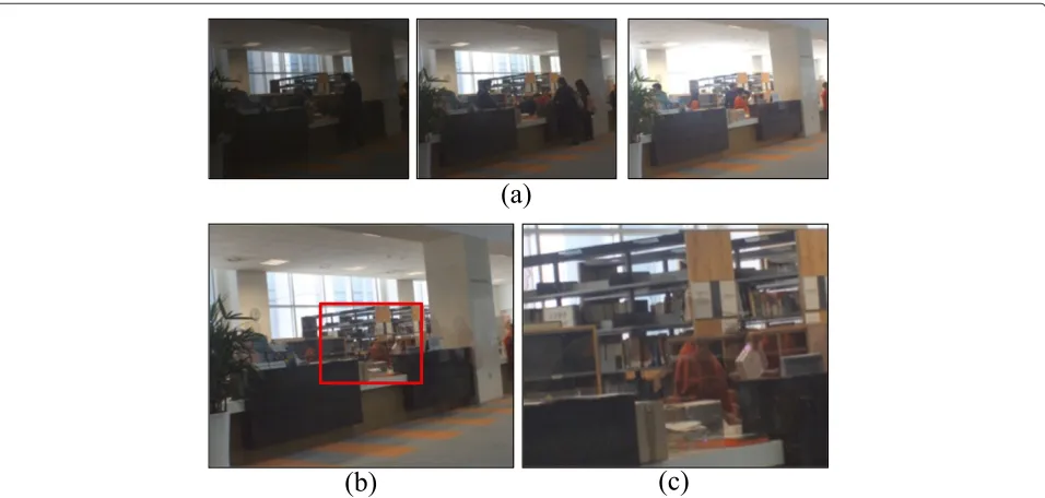
In general, any movement introduces ghost artifacts when input images with different exposures are sequentially acquired. Figure 7 shows the effect of these ghost artifacts. Figure 7a shows three input images with different expo-sures, and Figure 7b shows the HDR image result using a conventional Gaussian weight [11]. The movement of the people while the input images were being captured caused the ghost artifacts of the HDR image. The artifacts are shown in the close-up image (Figure 7c). To prevent the ghost artifacts, the region where local motion occurs has to be excluded from the reconstruction process.

The proposed method uses the weighting function to exclude the ghost artifacts. Small weights are assigned to the pixels where ghost artifacts occur to exclude the

ghosting regions from the reconstruction process. Before calculating the weighting function, the image with the fewest saturated and dark pixels is selected as the ence image. From the correspondence between the refer-ence image and the other BP-LDR images, the weighting functionW_nlis decomposed into the switching (sn) and the weighting (wl_n) components as

Wnli,j=sni,j·wl_ni,j. (15) The switching component sn is defined based on the fundamental assumption that the pixel value captured at a long exposure should be larger than that at a short expo-sure. Therefore, if the pixel value at a short exposure is larger than at a long exposure, this means that one of the two pixel values is wrong and should be excluded from the reconstruction process. Therefore,snbecomes

sni,j=

(a)

(b)

(c)

Figure 7An example of the ghost artifact in an HDR image.(a)Input images,(b)the result containing ghost artifact, and(c)close-up of the red box in(b).

wheren0denotes the reference image andMnrepresents the region inIn which satisfies the abovementioned fun-damental assumption. Even though the switching com-ponent is not used, the weighting comcom-ponentwl_nassigns small weights to these regions. However, the switching component is effective to reduce ghost artifacts because these regions are completely excluded from the recon-struction process by the switching component.

The weighting component wl_n is determined by the differences of the luminance and chrominance values between the reference image and the other BP-LDR images. The regions with large differences can be regarded as regions where local motion occur, and thus small weights have to be assigned to these regions. On the other hand, large weights have to be assigned to regions with small differences. The above description is applied towl_n, and it is assigned to the pixels as

wlni,j=exp−CY·DnYi,j−CR·DRni,j −CB·DBni,j.

(17)

Here,DY_n represents the difference of the luminance val-ues betweenIn0andIn.DXn, whereXdenotes the red (R) or

blue (B) channel, represents the difference of the chromi-nance values betweenIn0 andIn. The parametersCY,CR,

andCBare chosen to balance between DY_n,DR_n, and DB_n, respectively.

To obtain DY_n and DX_n, first, the BP-LDR images are adjusted to the same exposure setting because the expo-sures of the BP-LDR images differ. The procedure to

adjust the exposure can be expressed in terms of the formula below:

In1→n2 =min

f

f−1_I

n1

× tn2

tn1

,Imax

(18)

whereIn1→n2represents the imageIn1 of which the

expo-sure time changes from tn1 to tn2, and min{a,b}

represents the minimum value between a and b. From the exposure adjustment in (18), the exposure time of In1 changes fromtn1 totn2 in the radiance domain,

and then it is converted in the pixel value domain. After adjusting the exposures,DY_n is calculated as

DY ni,j=

Y˜n0

i,j− ˜Yni,j maxY˜n0

i,j,Y˜ni,j (19)

where

˜

Yni,j= (p,q)∈S

Gσ(p,q)·Yni+p,j+q. (20)

Here, max{a,b}represents the maximum value between a andb, Yn represents the luminance component of In, Gσ(·) represents the corresponding truncated Gaussian kernel with variance σ2, and S represents an index set of a support, i.e., a rectangular windowed search range. The normalization ofY˜n0

luminance. The luminance componentYnis calculated in the Bayer pattern from neighboring pixels as

Yni,j=1

4·In(i,j)+ 1 8·

In(i−1,j)+In(i,j−1) +In(i+1,j)+In(i,j+1)

+ 1 16·

In(i−1,j−1)+In(i−1,j+1) +In(i+1,j−1)+In(i+1,j+1).

(21)

By applying (21),Yn contains 50% green, 25% red, and 25% blue colors regardless of the position. DX_n is also calculated after adjusting the exposures as follows:

DXni,j= K˜X

n0

i,j− ˜K_nXi,j

maxY˜_nX₀i,j,Y˜_nXi,j (22)

whereK˜_nXis calculated by ˜

KX n i,j=

(p,q)∈S

Gσ(p,q)·Yni+p,j+q

−Xni+p,j+q.

(23)

Here,Xn represents the pixel value of the X channel in In, which is calculated by the bilinear interpolation depending on the position.

Figure 8 shows the results of obtaining DY_n, DR_n, and DB

n between the reference image (middle exposure) and the other two BP-LDR images. The regions where DY_n, DR

n, and DBn are large are regarded as the local motion regions. In Figure 8, it can be seen that the local motion is detected effectively. Although it is difficult to detect the local motion in the dark region of the short-exposure BP-LDR image due to the influence of the noise, there is no problem since the short-exposure BP-LDR image is rarely used to reconstruct dark regions of the scene.

2.2.3 The weight for data reliability considering local motion

If the weighting function W_nr obtained in the previous section asWˆ_nr in (3) is used, this will cause a problem: a certain local motion can cause artifacts. For easy under-standing, let us consider a situation in which two LDR images have different exposures. Suppose that the image with shorter exposure is the reference image. Figure 9 illustrates this situation. Here, the local motion region is shown in the longer exposure image I1 (marked by

light gray in Figure 9c), and the black region is shown in the shorter exposure image I2 (marked by dark gray in

Figure 9c). When calculatingWnforn= 1, 2 by (3) using Wr

n, they have weighting values W1 ≈ 0 and W2 ≈ 0,

respectively. This is due to the fact that the local motion

Y

D

Y

D

D

D

R

D

D

3

(a)

(b)

(c)

Figure 9An example of a situation in which the weighting functionsWnfor allnbecome 0.(a)A long-exposure imageI1,(b)a

short-exposure imageI2(reference image), and(c)a weight image (light gray:W1≈0, dark gray:W2≈0, black:W1,W2≈0).

region inI1leads toW1l ≈ 0, and the black region inI2

leads to W₂r ≈ 0. As a result, an artifact appears since no LDR images are utilized in the intersection of these two regions (marked by black in Figure 9c). To avoid the artifact, the weighting functionW_nrhas to be modified.

The modified weighting function Wˆ_nr should increase its weight if a local motion occurs in the opponent BP-LDR image to compensate for the small weighting value of the local motion region. For example, again, regarding the case where the imageI1is obtained with the longest

exposure, I2 with the second longest,I3 with the third,

and so on forIn=4,5,...,N. In this case, first, the weighting functionWˆ₁rfor the longest exposure BP-LDR imageI1is

composed ofW₁r and a partial weighting ofW₂r to com-pensate for the local motion inI2. In detail, when a local

motion is detected in a certain region inI2, a partial weight

ofW₂ris added toWˆ₁rfor this region. The modified weight ˆ

W1rdoes not include the partial weights ofWnr=3,...,N, since Wnr=3,...,N are almost 0 in the radiance value range ofI1.

Therefore,Wˆ₁rcan be expressed as follows:

ˆ

The weightW₂lis the weight defined in (15) for the case of imageI2. It has a small value if the likelihood of a local

motion inI2is large. IfW2l has a small value, the weight Wr

2is much reflected in the weightWˆ1r. The imageI1→2is

used to computeW₂r, whereI1→2is calculated from (18).

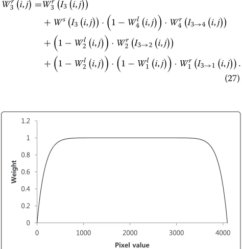
Here,Ws(·)represents a simple hat function [7] as shown in Figure 10, which prevents the use of saturated values in In:

same manner as explained in the abovementioned case.

Furthermore, the weight W₁r is additionally included in ˆ

W2r. This is due to the fact that the radiance range ofI2

includes the radiance range of I1, which is again due to

the fact thatI2is obtained with a shorter exposure thanI1.

Therefore, usingI2to compensate for the local motion in I1andI3,Wˆ2rbecomes

Here, the weightWsis not required for the third term in the right hand side of (26), since the radiance value range captured byI1corresponds to the low-radiance part ofI2.

Similarly, Wˆ₃r contains the weights W₃r, W₁r, W₂r, and

The fourth term compensates for the case if local motion is detected in bothI1andI2. If local motion occurs

only inI2, then the third term in (27) would be enough.

Otherwise, the case that local motion occurs only inI1is

already compensated for by the third term in (26). Generalizing the case forn(except forn = 1 andn =

Finally, the weighting functionWˆ_nr is used as the data reliability term in (3).

3 Experimental results

The performance of the proposed algorithm was tested with several BP-LDR images, which were captured with a CMOS sensor at three different exposures (t1 = t, t2 = t/4, andt3 =t/16). The BP-LDR images have a

pixel value range of 0 ≤ intensity ≤ 4, 095 (12-bit). The 12-bit pixel value range is widely used for digital cameras. Later, the 12-bit range is compressed to 8-bit RGB data by the IPM.

With the proposed method, several parameters were set empirically and tested with various images to obtain the best results. The parameterρin (5) was set to2₃Imax. The

parameter δ in (6), which determines the degree of the overlap between the data reliability weights, was set to 0.25. The parametersCY,CRandCBin (17) were set to 20, 10, and 10, respectively. The kernel sizeSand the variance σ2_{in (20) and (23) were set to 5×5 and 4, respectively.}

No pre-processes were performed on the input BP-LDR image, but pre-processes such as bad pixel correction [22] and Gr-Gb imbalance correction [23] can improve the HDR result according to the quality of the imaging sen-sor. For better visualization, we showed the results in RGB images rather than in Bayer patterned images. All the input BP-LDR images were post-processed by the edge-preserving color interpolation [24], white balancing, color correction, and gamma correction. For the resulting BP-HDR images, an additional tone-mapping algorithm [25] was used to compress the dynamic range, which visual-izes the HDR image information on a low dynamic range display.

We compared the performance with respect to the influ-ence of noise at dark regions and ghost artifacts with three conventional methods. The first conventional method

(CM1) uses the weighted summation using the Gaus-sian weighting function without considering ghost artifact reduction in [11]. The second (CM2) and third (CM3) method are commercial software programs that are widely used to obtain an HDR image with ghost artifact reduction in [26,27], respectively. In CM2 and CM3, the parame-ters associated with ghost artifact removal were set to the highest level. For CM2 and CM3, the BP-LDR images were preprocessed by the same edge-preserving color interpo-lation, white balancing, and gamma correction algorithms which are used for the visualization.

First, we performed an experiment when there was no local motion. Figure 11 shows our HDR result applied to a scene containing both indoor and outdoor environ-ments. As can be seen in Figure 11a, the limited dynamic range of the imaging sensor revealed saturation and black regions in the LDR images. In the short-exposure LDR image, the pixels in the bright regions avoided saturation, but the details in the dark regions disappeared. On the other hand, in the long exposure LDR image, the dark regions, e.g., the part under the desk, became visible, but the bright regions became saturated. In comparison, with the proposed method, the fine details became visible in both the bright and the dark regions, as can be seen in Figure 11b. Figure 11c visualizes the values of the weight-ing functionsWn=1,2,3in colors. The R, G, and B channels

were assigned toW1,W2, andW3, respectively. For

exam-ple, a red region represents the fact that the value ofW1is

dominant in that region. As a result, in the reconstruction of the BP-HDR image, the long-exposure BP-LDR image has a dominant effect on the region under the desk, while the short-exposure BP-LDR image has a dominant effect on the sky region.

(a)

(b)

(c)

Figure 11Experimental results of the captured scene with window.(a)The three LDR images,(b)the result of the proposed method, and(c)

the weight image obtained byWn.

(a)

)

c

(

)

b

(

)

e

(

)

d

(

)

b

(

)

a

(

)

d

(

)

c

(

Figure 13Close-up comparison of Figure 12.(a)CM1,(b)CM2,(c)CM3, and(d)the proposed method.

region revealed similar small weights for all the BP-LDR images. In comparison, with the proposed method, Wn assigned a dominant weight for the long-exposure BP-LDR image in the dark region, which made the dark region visible.

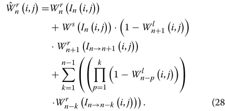
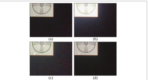
Figure 15 shows the results for a scene with a desk. The scene contained a very dark region under the desk as shown in Figure 15a. In Figure 15, it appears that the noise under the desk was reduced effectively in the results of the CM2 and the proposed method, while the CM1 and the CM3 did not reduce the influence of noise and even generated some artifacts in the light source. How-ever, with the CM2, the details in both the bright and dark regions were disappeared when compared with the

other results. To evaluate the performance with respect to the influence of noise, the standard deviation (σ) and the coefficient of variation (CV) were used as objective performance criteria. The CV is defined as the ratio of the standard deviationσ to the mean μ, i.e., σ/μ. The CV is useful for comparison when the means in the result images are different from each other. Table 1 presents the standard deviations and the CVs of the proposed method and the CMs, which are calculated in the homo-geneous dark regions of Figures 13 and 15. As described in Table 1, the PM recorded a smaller standard deviation and CV values than the CMs. From Table 1, it is clear that the proposed method outperforms the CMs in numerical values.

)

b

(

)

a

(

(a)

)

c

(

)

b

(

)

e

(

)

d

(

Figure 15Experimental results of the captured scene with desk.(a)The three LDR images,(b)CM1,(c)CM2,(d)CM3, and(e)the proposed method.

In the second experiment, we performed experiments on captured scenes that included object movements. Figure 16 shows the results for a scene with leaves blowing in the wind. Figure 16b shows the ghost artifacts around the leaves since CM1 cannot consider local motion. The CM2 cannot remove the ghost artifacts effectively, as can

Table 1 Comparison of experimental results in quantitative terms

Image Method σ CV

Chart CM1 9.61 0.475

CM2 11.96 0.478

CM3 12.06 0.334

Proposed 5.15 0.281

Desk CM1 7.51 0.225

CM2 5.94 0.467

CM3 7.43 0.273

Proposed 4.91 0.220

be seen in Figure 16c. Figure 16d,e shows the results when using the CM3 and the proposed method, respectively. Both results show almost no ghost artifacts when com-pared with the results of the CM1 and the CM2. As a result, the CM3 and the proposed method are able to pre-vent ghost artifacts from small local motion like blowing leaves.

(a)

(b)

(c)

(d)

(e)

Figure 16Experimental results of the captured scene with leaves blowing in the wind.(a)The three LDR images,(b)the result of CM1,(c)the result of CM2,(d)the result of CM3, and(e)the result of the proposed method.

(a)

)

d

(

)

c

(

(b)

)

d

(

)

c

(

)

a

(

(b)

Figure 18Close-up comparison of Figure 17.(a)The result of CM1,(b)the result of CM2,(c)the result of CM3, and(d)the result of the proposed method.

result, false colors may occur in the achromatic regions. Moreover, as can be seen in Figure 18, conventional meth-ods cannot detect the person wearing black pants in front of the black desk because their brightness values are sim-ilar. In comparison, the proposed method prevents ghost artifacts and produces a high-quality BP-HDR image, as shown in Figure 18d.

We presented the results of the proposed method together with the input images in Figure 19. Figure 19

demonstrates that the proposed method provides BP-HDR images without any artifacts.

4 Conclusion

In this paper, we have proposed a BP-HDR (Bayer patterned high dynamic range) image reconstruction algorithm from multiple BP-LDR (Bayer patterned low dynamic range) images. Unlike conventional methods, the proposed method works on the Bayer raw image. This

allows for a linear CRF and also improves the efficiency in hardware implementation. The proposed method aims to deal with the noise and the ghost artifact problems. For this aim, a new weighting function is proposed to be designed so that each of the BP-LDR images indepen-dently covers its corresponding region according to the radiance value. Furthermore, the weighting function is designed to detect the local motion in the Bayer pattern and to exclude ghosting regions. As a result, the proposed method weakens the influence of noise in the short-exposure BP-LDR image and prevents ghost artifacts. Experimental results show that the proposed method pro-duces a high-quality BP-HDR image while being robust against ghost artifacts and noise factors, even when there exists excessive local motion.

Appendix

Procedure for calculating intersection pointγn

The intersection pointγnofW˜_nr andW˜_nr₊₁is determined as the same point obtained from the conventional weight-ing function. We use the simple weightweight-ing function to calculateγnas

Wc

The weighting functionW_ncis shown in the top part of Figure 4. The falling part of W_nc and the rising part of Wc

n+1intersect in the radiance domain. The procedure for

calculating the intersection pointγnis shown below:

−1

The authors declare that they have no competing interests.

Acknowledgements

This work was supported by the National Research Foundation of Korea (NRF) grant funded by the Korea government (MSIP) (No. 2012R1A2A4A01003732).

Author details

1_{Department of Electric and Electronic Engineering, Yonsei University, 50}

Yonsei-ro, Seodaemun-gu, Seoul 120-749, Korea.2_{Department of Multimedia}

Engineering, Dongseo University, 47 Jurye-ro, Sasang-gu, Busan 617-716, Korea.

Received: 5 February 2014 Accepted: 5 May 2014 Published: 22 May 2014

References

1. S Mann, R Picard, Being ‘undigital’ with digital cameras: extending dynamic range by combining differently exposed pictures, inIS&T 48th Annual Conference(Washington D.C., 7–11 May 1995), pp. 422–428 2. T Mitsunaga, SK Nayar, Radiometric self calibration, in1999 IEEE Computer

Society Conference on Computer Vision and Pattern Recognition, vol. 1 (Fort Collins, 23–25 June 1999), pp. 374–380

3. PE Debevec, J Malik, Recovering high dynamic range radiance maps from photographs, in24th International Conference on Computer Graphics and Interactive Techniques(Los Angeles, 3–8 Aug 1997), pp. 369–378 4. C Pal, R Szeliski, M Uyttendaele, N Jojic, Probability models for high

dynamic range imaging, in2004 IEEE Computer Society Conference on Computer Vision and Pattern Recognition, vol. 2 (Washington D.C., 27 June–2 July 2004), pp. 173–180

5. A Srikantha, D Sidibé, Ghost detection and removal for high dynamic range images: recent advances. Signal Process. Image Commun. 27(6), 650–662 (2012)

6. O Gallo, N Gelfandz, W-C Chen, M Tico, K Pulli, Artifact-free high dynamic range imaging, in2009 IEEE International Conference on Computational Photography(San Francisco, 16–17 Apr 2009), pp. 1–7

7. EA Khan, AO Akyuz, E Reinhard, Ghost removal in high dynamic range images, in2006 IEEE International Conference on Image Processing(Atlanta, 8–11 Oct 2006), pp. 2005–2008

8. K Jacobs, C Loscos, G Ward, Automatic high-dynamic range image generation for dynamic scenes. IEEE Trans. Comput. Graphics Appl. 28(2), 84–93 (2008)

9. YS Heo, KM Lee, SU Lee, Y Moon, J Cha, Ghost-free high dynamic range imaging, in10th Asian Conference on Computer Vision, vol. 6495 (Queenstown, 8–12 Nov 2010), pp. 486–500

10. J An, SH Lee, JG Kuk, NI Cho, A multi-exposure image fusion algorithm without ghost effect, in2011 IEEE International Conference on Acoustics, Speech and Signal Processing(Prague, 22–27 May 2011), pp. 1565–1568 11. MA Robertson, S Borman, RL Stevenson, Dynamic range improvement through multiple exposures, in1999 International Conference on Image Processing, vol. 3 (Kobe, 24–28 Oct 1999), pp. 159–163

12. L Shao, AU Rehman, Image demosaicing using content and colour-correlation analysis. Signal Process. doi: 10.1016/j.sigpro. 2013.07.017

13. L Shao, H Zhang, G de Haan, An overview and performance evaluation of classification-based least squares trained filters. IEEE Trans. Image Process. 17(10), 1772–1782 (2008)

14. R Ramanath, WE Snyder, Y Yoo, MS Drew, Color image processing pipeline. Signal Process. Mag. IEEE.22(1), 34–43 (2005)

15. L Shao, R Yan, X Li, Y Liu, From heuristic optimization to dictionary learning: a review and comprehensive comparison of image denoising algorithms. IEEE Trans. Cybernet. doi:10.1109/TCYB.2013.2278548 16. B Pham, G Pringle, Color correction for an image sequence. Comput.

Graphics Appl. IEEE.15(3), 38–42 (1995)

17. BE Bayer, Color imaging array. U.S. Patent 3,971,065, July 1976 18. GC Holst, TS Lomheim,CMOS/CCD Sensors and Camera Systems, 2nd edn.

(SPIE, Bellingham, 2011)

19. MD Grossberg, SK Nayar, Determining the camera response from images: what is knowable? IEEE Trans. Pattern Anal. Mach. Intell.25(11), 1455–1467 (2003)

20. Y Tsin, V Ramesh, T Kanade, Statistical calibration of, CCD imaging process, in8th IEEE International Conference on Computer Vision, vol. 1 (Vancouver, 7–14 July 2001), pp. 480–487

21. YS Han, E Choi, MG Kang, Smear removal algorithm using the optical black region for CCD imaging sensors. IEEE Trans. Consum. Electron. 55(4), 2287–2293 (2009)

22. B Dierickx, G Meynants, Missing pixel correction algorithm for image sensors, inEUROPTO Conference on Advanced Focal Plane Arrays and Electronic Camera 2(Zurich, 7 Sep 1998), pp. 200–203

23. N Chino, H Une, Color imaging by independently controlling gains of each of R, Gr, Gb, and B signals. U.S. Patent 7,009,639, March 2006 24. W Lu, Y-P Tan, Color filter array demosaicking: new method and

25. L Meylan, S Susstrunk, High dynamic range image rendering with a retinex-based adaptive filter. IEEE Trans. Image Process.15(9), 2820–2830 (2006)

26. Photomatix Version 4.0.2, HDRsoft http://www.hdrsoft.com/. Accessed 31 Jan 2014

27. Adobe Photoshop CS5 Version 12.0.4. Adobe Systems Inc. http://www. adobe.com/products/photoshop/. Accessed 31 Jan 2014

doi:10.1186/1687-6180-2014-76

Cite this article as:Kanget al.:Bayer patterned high dynamic range image reconstruction using adaptive weighting function.EURASIP Journal on Advances in Signal Processing20142014:76.

Submit your manuscript to a

journal and benefi t from:

7Convenient online submission

7Rigorous peer review

7Immediate publication on acceptance

7Open access: articles freely available online

7High visibility within the fi eld

7Retaining the copyright to your article