Evolution of dust grain size distribution by shattering in the interstellar
medium: Robustness and uncertainty
Hiroyuki Hirashita1and Hiroshi Kobayashi2
1Institute of Astronomy and Astrophysics, Academia Sinica, P.O. Box 23-141, Taipei 10617, Taiwan 2Department of Physics, Nagoya University, Nagoya, Aichi 464-8602, Japan
(Received November 16, 2012; Revised February 27, 2013; Accepted March 9, 2013; Online published October 24, 2013)
Shattering of dust grains in the interstellar medium is a viable mechanism of small grain production in galaxies. We examine the robustness or uncertainty in the theoretical predictions of shattering. We identifyP1(the critical pressure above which the deformation destroys the original lattice structures) as the most important quantity in determining the timescale of small grain production, and confirm that the same P1/t (t is the duration of shattering) gives the same grain size distribution [n(a), where a is the grain radius] after shattering within a factor of 3. The uncertainty in the fraction of shocked material that is eventually ejected as fragments causes uncertainties in n(a) by a factor of 1.3 and 1.6 for silicate and carbonaceous dust, respectively. The size distribution of shattered fragments have minor effects as long asαf 3.5 (the size distribution of shattered fragments∝a−αf), since the slope of grain size distributionn(a)continuously changes by shattering and becomes
consistent withn(a) ∝ a−3.5. The grain velocities as a function of grain radius can have an imprint in the grain size distribution especially for carbonaceous dust. We also show that the formulation of shattering can be simplified without losing sufficient precision.
Key words:Cosmic dust, galaxy evolution, grain size distribution, interstellar medium.
1.
Introduction
The evolution of dust in galaxies is important to the understanding of galaxy evolution, since dust grains gov-ern some fundamental physical processes in the interstel-lar medium (ISM). First, they dominate the absorption and scattering of the stellar light, affecting the radiative transfer in the ISM. Second, the dust surface is the main site for the formation of molecular hydrogen. The former process is governed by the extinction curve (absorption and scat-tering coefficient as a function of wavelength; Hoyle and Wickramasinghe, 1969; Draine, 2003) and the latter by the total surface area of dust grains (Yamasawaet al., 2011). Since the extinction curve and the total grain surface area both depend strongly on the grain size distribution, clarify-ing the regulatclarify-ing mechanism of grain size distribution is of particular importance in understanding those important roles of dust.
Mathiset al. (1977, hereafter MRN) show that a mixture of silicate and graphite with a grain size distribution [num-ber density of grains per grain radius, denoted asn(a)in this paper] proportional toa−3.5(a grain size distribution with a power index of−3.5 is called MRN grain size distribution), wherea is the grain radius (a ∼ 0.001–0.25μm), repro-duces the Milky Way extinction curve. Pei (1992) shows that the extinction curves in the Magellanic Clouds are also explained by the MRN grain size distribution with different
Copyright cThe Society of Geomagnetism and Earth, Planetary and Space Sci-ences (SGEPSS); The Seismological Society of Japan; The Volcanological Society of Japan; The Geodetic Society of Japan; The Japanese Society for Planetary Sci-ences; TERRAPUB.
doi:10.5047/eps.2013.03.008
abundance ratios between silicate and graphite. Kimet al. (1994) and Weingartner and Draine (2001) have applied a more detailed fit to the Milky Way extinction curve in order to obtain the grain size distribution. Although their grain size distributions deviate from the MRN size distribution, the overall trend from small to large grain sizes roughly fol-lows a power law with an index near to−3.5. In any models that fit the Milky Way extinction curve, the existence of a large number of small (a 0.01μm) grains is required. The existence of such small grains is further supported by the mid-infrared excess of the spectral energy distribution in the Milky Way (e.g., D´esertet al., 1990; Draine and Li, 2001).
Dust grains formed by stellar sources, mainly supernovae (SNe) and asymptotic giant branch (AGB) stars, are not sufficient to explain the total dust mass in the Milky Way ISM, because the timescale of dust enrichment by these sources is much longer than that of dust destruction by SN shocks (e.g., McKee, 1989; Draine, 1995). Moreover, both SNe and AGB stars are suggested to supply large (a 0.1μm) grains into the ISM and cannot be the dominant source of small grains (Nozawaet al., 2007; H¨ofner, 2008; Mattsson and H¨ofner, 2011; Norris et al., 2012). Thus, some interstellar processes (or more precisely, non-stellar processes) are necessary to explain the large abundance of small grains.
There are some possible processes that efficiently mod-ify the grain size distribution. Hellyer (1970) shows that the collisional fragmentation of dust grains finally leads to a power-law grain size distribution similar to the MRN size distribution (see also Bishop and Searle, 1983; Tanaka
et al., 1996). Hirashita and Yan (2009) show that such a fragmentation and disruption process (or shattering) can be driven efficiently by turbulence in the diffuse ISM. Dust grains are also processed by other mechanisms. Various authors show that the increase of the total dust mass in the Milky Way ISM is mainly governed by grain growth through the accretion of gas phase metals onto the grains (we call elements composing dust grains “metals”) (e.g., Dwek, 1998; Zhukovskaet al., 2008; Inoue, 2011; Asano et al., 2013a). Grain growth mainly works in the dense ISM, such as molecular clouds. In the dense ISM, coag-ulation also occurs, making the grain sizes larger (e.g., Hi-rashita and Yan, 2009; Ormelet al., 2009). In the diffuse ISM phase, interstellar shocks associated with supernova (SN) remnants destroy dust grains, especially small ones, by sputtering (e.g., McKee, 1989; Nozawa et al., 2006). Shattering also occurs in SN shocks (Joneset al., 1996). All these processes above other than shattering do not con-tribute efficiently to the increase of small (a 0.01μm) grain abundance. Indeed, Asanoet al. (2013b) show that, unless we consider shattering, the grain size distribution is biased to large (a ∼0.1μm) sizes. Therefore, shattering is important in reprocessing large grains into small grains.
Based on the formulation developed by Hirashita and Yan (2009), Hirashitaet al.(2010, hereafter H10) consider small grain production by shattering in the context of galaxy evolution. H10 assume that Type II SNe (SNe II) are the source of the first dust grains, which are biased to large sizes (0.1μm) because small grains are destroyed in the shocked region in the SNe II (Nozawaet al., 2007, hereafter N07). Starting with the size distribution of SNe II dust grains in N07, H10 solve the shattering equation to calculate the evolution of grain size distribution. They show that the velocity dispersions acquired by the dust grains in a warm ionized medium (WIM) is large enough for shattering to produce a large abundance of small grains on a short (10 Myr) timescale. As mentioned above, even if we consider other sources of dust such as the dust formation in the wind of AGB stars and the accretion of metals onto grains in the interstellar clouds, shattering is generally necessary to produce small grains (Asanoet al., 2013b).
Considering that shattering is a unique mechanism that produces small grains efficiently in the ISM, it is important to clarify how robust or uncertain the theoretical calcula-tions of shattering are. Since there are some basic physical parameters regulating shattering, it is crucial to clarify how they affect the grain size distribution or to which parameter shattering is sensitive. Although any models should com-monly contain those basic parameters, there could be some uncertainties in the formulation itself, or there could be un-necessary complexity which cannot be constrained from ob-servations anyway. Thus, in this paper, we examine the ro-bustness of shattering calculations for the interstellar dust by changing some major parameters in a model and com-paring the results between two different frameworks.
This paper is organized as follows. In Section 2, we ex-plain the shattering models and pick out some major param-eters. In Section 3, we examine the variation of the grain size distribution due to changes of the major parameters. In Section 4, we discuss our results and implications for the
evolution of grain size distribution. In Section 5, we give our conclusions.
2.
Overview of the Models for Shattering
As mentioned in Introduction, we use the framework in H10 to test the robustness of a shattering model. H10 consider the evolution of grain size distribution through shattering by solving a shattering equation, which treats the grain–grain collision rate and the redistribution of shattered fragments in the grain size distribution. They assume that grains collide with each other under the velocity dispersions induced by dynamical coupling with interstellar turbulence. The production of fragments in grain–grain collisions is the key process that we focus on below.
The dust grains are assumed to be spherical with radius a. Thus, the grain massmis related to the grain radius by
m= 4 3πa
3ρ
gr, (1)
whereρgris the material density of the grain. The grain size distribution,n(a), is defined so thatn(a)dais the number density of grains with radii betweenaanda+da.
2.1 Initial grain size distribution
The size distribution of grains ejected from SNe II into the ISM is adopted from N07. This size distribution is used as the initial condition for the calculation of shatter-ing. N07 treated dust nucleation and growth in a SN II, taking into account the dust destruction by kinetic and ther-mal sputtering in the shocked region. Thus, the grain size distribution calculated by N07 is regarded as that ejected from SNe II to the ISM (see also Bianchi and Schneider, 2007). Following H10, we adopt 20 Mas a representative progenitor mass, and the unmixed case in which the origi-nal onion-like structure of elements is preserved, since the extinction features of carbon and silicon, which are major grain components in the unmixed case, are consistent with observations (Hirashitaet al., 2005; Kawaraet al., 2011). The formed grain species are C, Si, SiO2, Fe, FeS, Al2O3, MgO, MgSiO3, and Mg2SiO4. According to N07, small grains witha 0.02μm are trapped in the shocked re-gion and are efficiently destroyed by thermal sputtering if the ambient hydrogen number density,nH, is larger than 0.1 cm−3. In this paper, we adoptn
H = 1 cm−3 (Subsection 2.2). As shown in N07 (see also H10), most of the grains have radii 0.1–1μm. The initial grain size distributions are also shown later in Fig. 2.
Table 1. Summary of experimental properties.
Note: All the quantities are determined experimentally. See Joneset al.(1996) and references therein.
size distribution is normalized so that the total grain mass density integrated for all the size range, ρdust, is equal to 1.4nHmHD0, wheremHis the mass of hydrogen atom, and the factor 1.4 is the correction for the species other than hy-drogen.
As mentioned in Introduction, additional contribution from AGB stars does not change the following results sig-nificantly as long as AGB stars also supply large (a 0.1 μm) grains (see also Asano et al., 2013b). In other words, the use of N07’s results for the initial condition is aimed at investigating the important role of shattering in the production of small grains from large grains.
2.2 Shattering
We calculate the shattering processes in the same way as in H10 by solving the shattering equation. The collision fre-quency between grains with various sizes is determined by grain-size-dependent velocity dispersions. The shattering equation used in H10 is based on Hirashita and Yan (2009) (originally taken from Joneset al., 1994, 1996). Shattering is assumed to take place if the relative velocity between a pair of grains is larger than the shattering threshold veloci-ties,vshat(2.7 and 1.2 km s−1 for silicate and graphite, re-spectively; Joneset al., 1996). The results are not sensitive tovshatas long as the grain velocities driven by turbulence is much larger than the threshold, but are rather sensitive to the hardness of the grain materials as shown later.
We consider a range amin = 3×10⁻⁸ cm (3 ˚A) and amax = 3 ×10⁻⁴ cm (3 μm) for the grain radii. The grains passing through the boundary of the smallest radius are removed from the calculation. Most grain models adopt a minimum grain radius of a few×10−8 cm (Weingartner and Draine, 2001; Guilletet al., 2009) although applying bulk material properties to such small grains could cause a large uncertainty. However, even if we adopt amin = 10−7cm, the results does not change, except that the grain size distribution is truncated at 10−7 cm. This is because shattering occurs in a top-down manner in the grain sizes and the production of grains witha ∼a few×10−8cm by shattering is never enough for these small grains to have a large contribution to the total shattering rate.
Although nine grain species are predicted to form (Sub-section 2.1), the material properties needed for the calcu-lation of shattering are not necessarily available for all the species. Thus, we divide the grains into two groups: one is carbonaceous dust and the other is all the other species of dust (called “silicate”), and apply the relevant material quantities of graphite and silicate, respectively. The mate-rial properties of silicate and graphite are taken from Jones et al. (1996) and summarized in Table 1.
Since the shattering equation is general enough, the ma-jor uncertainties can be produced by the treatment of
shat-tering fragments. Thus, we explain how to treat shatshat-tering fragments below.
We consider two colliding grains whose masses arem1 andm2 (the former grain is called target grain), and esti-mate the total fragment mass inm1as a result of this col-lision. Note that we consider a collision betweenm2 and m1 again in the calculation and consider the fragments in m2(that is, we consider the same collision twice to treat the fragments of each colliding grain). The total fragment mass is determined by the mass shocked to the critical pressure in the target (Joneset al., 1996; Hirashita and Yan, 2009):
Mej
whereMejis the total mass of fragments ejected fromm1, M is the mass shocked to the critical pressure (P1), above which the solid becomes plastic (that is, the deformation destroys the original lattice structures), fM is the fraction
of shocked mass that is eventually ejected as fragments (the rest remains in the grain),R =1 in the collision between the same species (we only consider collisions between the same species for simplicity),Mr ≡ v/c0(c0 is the sound speed of the grain material),M1is the Mach number cor-responding to the critical pressureP1:
M1= 2φ1 1+(1+4sφ1)1/2
, (3)
whereφ1 ≡ P1/(ρgrc20)andsis a dimensionless material constant that determines the relation between the shocked velocity and the velocity of the shocked matter. For conve-nience, we define functionσ as
σ (M)≡ 0.30(s+M−1−0.11)1.3
s+M−1−1 , (4)
and evaluateσ1 = σ(M1)andσr = σ(Mr/(1+R))in
Eq. (2). IfM is larger than half of the grain mass, we as-sume that the whole grain is fragmented; i.e., Mej = m1. This case is called catastrophic disruption. Otherwise (i.e., for M < m1/2), only a fraction of m1 (fMM) is ejected
as fragments. This case is called cratering. The relation between the total volume (V) of shattered fragments and the critical pressure is roughly given by the total energy P1V = constant. Indeed, the above equations tell us that M ∝ V is inversely proportional to P1, if 4sφ1 > 1, which is true for most of the cases considered in this paper (M2
1∼φ1, soMej∝φ1−8/9 ∝ P −8/9
Table 2. Models.
Name Species fM P1 αf Grain velocities
(dyn cm−2)
Aa silicate 0.4 3×10¹¹ 3.3 Yanet al. (2004)
graphite 0.4 4×10¹⁰ 3.3 Yanet al. (2004)
B silicate 0.3 3×10¹¹ 3.3 Yanet al. (2004)
graphite 0.3 4×10¹⁰ 3.3 Yanet al. (2004)
C silicate 0.6 3×10¹¹ 3.3 Yanet al. (2004)
graphite 0.6 4×10¹⁰ 3.3 Yanet al. (2004)
Da silicate 0.4 1×10¹¹ 3.3 Yanet al. (2004)
graphite 0.4 1.3×10¹⁰ 3.3 Yanet al. (2004)
Ea silicate 0.4 9×10¹¹ 3.3 Yanet al. (2004)
graphite 0.4 1.2×10¹¹ 3.3 Yanet al. (2004)
F silicate 0.4 3×10¹¹ 2.3 Yanet al. (2004)
graphite 0.4 4×10¹⁰ 2.3 Yanet al. (2004)
G silicate 0.4 3×10¹¹ 4.3 Yanet al. (2004)
graphite 0.4 4×10¹⁰ 4.3 Yanet al. (2004)
H silicate 0.4 3×10¹¹ 3.3 Eq. (10)
graphite 0.4 4×10¹⁰ 3.3 Eq. (10)
aWe also examine KT10’s formulation for fragments (Section 2.4.2).
The total fragment mass Mej is distributed with a grain size distribution ∝ a−αf. Jones et al. (1996) argue that αf = 3.0–3.4, based on an analysis of the flow associ-ated with the formation of a crater (see also Takagiet al., 1984; Nakamura and Fujiwara, 1991; Nakamura et al., 1994; Takasawaet al., 2011 for experimental results). Un-less the catastrophic disruption occurs, we assume that the massm1−Mejremains as a single dust grain and is dis-tributed in an appropriate bin in the numerical calculation. To avoid unnecessary complexity caused by the choice of the upper and lower radii of the fragments, we adopt sim-pler forms for the smallest and largest fragments than H11, following Guilletet al. (2009):
afmax=(0.0204f)1/3a1, (5)
wherea1is the radius of the grainm1(i.e., the target grain), f ≡ Mej/m1 (shattered fraction of the target grain). The minimum radius is assumed to beaf,min = amin = 3× 10⁻⁸cm. Ifa
f,max <amin, we remove the fragments from the calculation.
The relative velocity in the collision is estimated based on the grain velocity dispersion as a function of grain radiusa. We used the calculation by Yanet al.(2004), who consider the grain acceleration by hydrodrag and gyroresonance in magnetohydrodynamic turbulence, and calculate the grain velocities achieved in various phases of ISM. Among the ISM phases, we focus on the warm ionized medium (WIM) to investigate the possibility of efficient shattering in ac-tively star-forming environments. We adoptnH =1 cm−3 for the hydrogen number density of the WIM. The resulting grain size distribution is not sensitive tonH(H10). Indeed, ifnHis large, the grain–grain collision rate (i.e., the shatter-ing efficiency) rises, while dust grains are more destroyed in SNe (i.e., the dust-to-gas ratio is lower). Because of these compensating effects, the resulting grain size distribution is not sensitive to the gas density. We adopt gas temperature T = 8000 K, electron number density ne = nH, Alfv´en speedVA=20 km s−1and injection scale of the turbulence
L = 100 pc. For grains with a 0.1 μm, where most of the grain mass is contained in our cases, the grain ve-locity is governed by gyroresonance. Since there is still an uncertainty in the typical grain radius (ac) above which gy-roresonance effectively works, we also address the variation of results byac(Subsection 2.4.4).
The grain velocities given above are velocity dispersions. In order to estimate the relative velocity (v12) between the grains withm1 andm2, whose velocity dispersions arev1 andv2, respectively, and we average the size distributions of fragments for four casesv12=v1+v2,|v1−v2|,v1, and
v2to take the directional variety into account. See H10 for more details.
2.3 Duration of shattering
Since we consider shattering in the WIM, it is reasonable to assume that the shattering duration (denoted ast) is deter-mined by a timescale on which the ionization is maintained. A typical lifetime of ionizing stars is10 Myr (Bressanet al., 1993; Inoueet al., 2000). We basically adoptt = 10 Myr in this paper, but we also consider longer durations for a longer starburst duration or shattering over multiple star-burst episodes.
2.4 Parameters
Based on the discussions in the previous subsection, we change the following parameters related to the fragments. The models are summarized in Table 2, where Model A adopts “fiducial” values for the parameters.
2.4.1 Ejected fraction of shocked material How much fraction of the shocked material is finally ejected as fragments is uncertain. This factor is denoted as fM in
Eq. (2). According to Joneset al. (1996), fM is between
0.3 and 0.6, while H10 adopted 0.4. Thus, we adopt 0.4 as a fiducial value (Model A) and also examine 0.3 (Model B) and 0.6 (Model C).
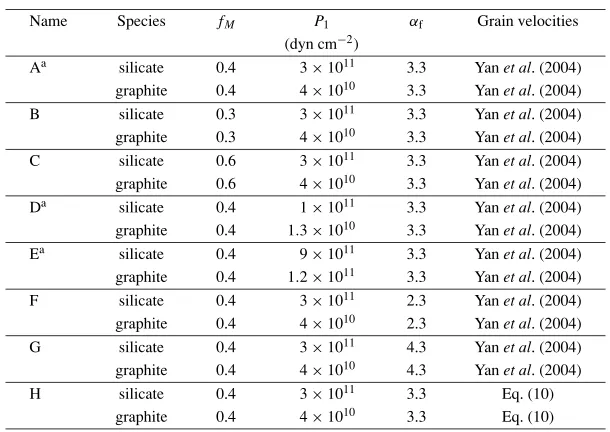
Fig. 1. Grain velocitiesvas a function of grain radiusa. Two grain species, (a) silicate and (b) carbonaceous dust, are shown. The solid lines indicate the velocity calculated by Yanet al. (2004) with the physical condition of the WIM described in the text. The dashed line shows the simplified velocity model (Eq. (10)) withac=10−6cm. The dotted line shows the shattering threshold velocity.
P1 = 3×10¹¹ and 4×10¹⁰ dyn cm−2 for silicate and graphite, respectively (Table 1; Model A in Table 2). We adopt three times smaller and larger values forP1in Models D and E, respectively. We call grains with low/high P1 soft/hard grains.
There is another possible way of including the criti-cal pressure in the model based on Kobayashi and Tanaka (2010, hereafter KT10). Jones et al. (1996) constructed the fragmentation model based on shock wave propagation caused by a collision (see also Mizutaniet al., 1990). On the other hand, Holsapple (1987) provided a scaling formula for collisional outcomes based on laboratory experiments of his group (the review of the scaling formula is seen in Holsap-ple, 1993). In this formula,Mejis proportional to
ϕ= Eimp m1QD
(6)
forϕ1, where
Eimp = 1 2
m1m2 m1+m2v
2 (7)
is the impact energy between m1 andm2, and QD is the specific impact energy atMej=m1/2. SinceMej∼m1for
ϕ 1, KT10 simply connected the cases forϕ 1 and
ϕ1, providing a simple formula forMejas
Mej=
ϕ
1+ϕm1. (8)
Now we relate QD to P1. The dominant channel for the small grain production is cratering of large grains by small grains. If we assume that m1 m2 (and as long asv2/Q
Dis not much larger than unity), we obtainMej m2v2/(2QD). On the other hand, if we approximate Eq. (2) as Mej/m2 A(ρgrv2/P1), A ∼ 1 for the range of quantities in this paper. Therefore, if the two models are equivalent,QD∼P1/(2ρgr).
Thus, we examine KT10’s formulation as follows. We adopt Eq. (8) instead of Eq. (2) for the total mass of frag-ments with the same fragment size distribution (∝a−αfwith
the same upper and lower grain radii). The value ofϕ is evaluated by Eqs. (6) and (7), whereQDis given by
QD= P1 2ρgr
. (9)
This equation indicates that, if the energy per unit volume given to the grain exceeds∼ P1/ρgr, the major part of the grain is disrupted. We test Models A, D, and E by adopting KT10’s formulation.
Note that we have adopted the approximation, Mej ∼
ρgrv2/P1. This is a good approximation for 4sφ1 > 1 (φ1 = P1/(ρgrc20); see Subsection 2.2). However, ifφ1 1, Mej/m2 ∼ (ρgrv2/P1)/φ1 for Eq. (2), so that QD =
(P1/2ρgr)φ1 gives a better approximation forφ1 1. In other words, ifφ1 is significantly smaller than 1 (i.e., for soft dust), Eq. (9) overestimatesQDby a factor ofφ1. Thus, if we calculate shattering by adopting Eq. (9), grains are shattered less compared with Jones et al.’s case for soft dust. In this paper, because it is easy to interpret Eq. (9), we simply adopt it for KT10’s formulation.
2.4.3 Size distribution of shattered fragments The power index of the size distribution of shattered fragments,
αf, may be reflected in the grain size distribution after shat-tering. The canonical value adopted in H10 isαf = 3.3, which is based on Joneset al. (1996). Here we also exam-ine the cases ofαf=2.3 and 4.3 (Models F and G, respec-tively), considering a wide range obtained in experiments (Takasawaet al., 2011).
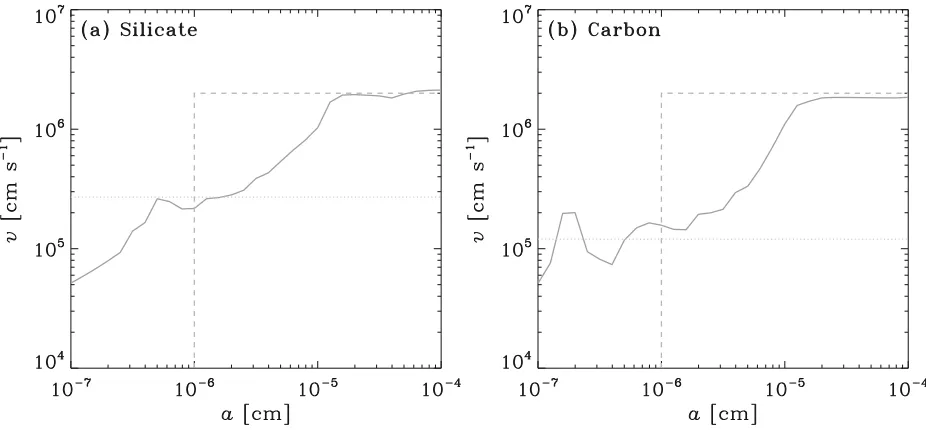
Fig. 2. Grain size distributions presented by multiplyinga4to show the mass distribution in each logarithmic bin of the grain radius. The solid, dashed, and dot-dashed lines show the results att =10 Myr for Models A, B, and C (fM =0.4, 0.3, and 0.6), respectively. The dotted line presents the
initial grain size distribution before shattering. Two grain species, (a) silicate and (b) carbonaceous dust, are shown. We also show a slope of 0.5 [i.e.,
n(a)∝a−3.5].
are coupled with larger-scale turbulence, the motions of larger grains are less affected by the damping by dissipa-tion, which occurs on small scales. The dissipation scale depends on the physical condition of the ISM, especially on the ionization degree. Thus, the critical grain size, above which the grains are efficiently accelerated by gyroreso-nance, varies by the physical condition of the ISM and the power spectrum of the turbulence. Because of such a vari-ation of the critical grain size, it is worth investigating how the shattered grain size distribution changes as a result of the variation of the critical grain size.
To make clear the dependence of the critical grain size denoted asac, we also examine a model in which the size dependence of the grain velocity dispersion is simplified as
v(a)=
vgyroifa≥ac, 0 ifa <ac.
(10)
An example withac=10−6cm is shown in Fig. 1. We fix
vgyro =20 km s−1. As long asvgyro > vsh, the variation of
vgyrochanges the timescale of shattering, which is roughly scaled with v−gyro1 . We examineac = 10−5 and 10−6 cm. This treatment of velocities is labeled as Model H.
3.
Results
3.1 Ejected fraction of shocked material
We examine the effect of fM on the grain size
distri-bution. In Fig. 2, we show the grain size distributions at t=10 Myr for Models A, B, and C. In this paper, the grain size distributions are presented by multiplyinga4 to show the mass distribution in each logarithmic bin of the grain radius. We observe that the production of small grains is
the most efficient for the largest fM. This is simply
be-cause a larger fraction of the shocked material is ejected as fragments. However, the abundance of the smallest grains is not simply proportional to fM, since the catastrophic
dis-ruption does not depend on fM. The maximum ratio ofn(a)
between fM =0.3 and 0.6 is 1.3 for silicate and 1.6 for
car-bonaceous dust.
3.2 Critical pressure
We examine the dependence on the critical pressure (P1). The adopted values for the fiducial case (Model A) is shown in Table 2, while smaller and larger values for P1 are also examined (Models D and E, respectively). In Fig. 3, we compare Models A, D, and E att =10 Myr. We find that the effect ofP1is significant. Carbonaceous dust in Model D has the lowestP1, so that the largest grains are efficiently shattered into smaller sizes. The mass loss rate of large grains with massm is proportional to P1−8/9 (Subsection 2.2); hence a lowP1increases the number density of small (a 10−6 cm) grains. On the other hand, collisional cascades determine the slope of the grain size distribution as−3.5, independent of P1 (Hellyer, 1970; Tanakaet al., 1996; KT10). The slope is therefore given by −3.5 for a 10−6 cm, a value (−3.5) consistent with one derived observationally for the dust grains in the Milky Way and the Magellanic Clouds (Mathiset al., 1977; Pei, 1992).
Fig. 3. Same as Fig. 2 but for Models A, D, and E. The thick solid, dashed, and dot-dashed lines show the results att =10 Myr for Models A, D, and E (fiducial, hard, and soft grains), respectively, while the thin lines adopt the treatment of fragments by KT10 (the same line species shows the same model). The dotted line presents the initial grain size distribution before shattering. Two grain species, (a) silicate and (b) carbonaceous dust, are shown.
E), but the discrepancy is relatively large for the soft dust (Model D) because Eq. (9) is not a good approximation for the soft dust (see Subsection 2.4.2 for detailed discussions). The maximum ratio between the two formulations in Model D is 1.8 for silicate and 2.2 for carbonaceous dust. For car-bonaceous dust, the maximum difference occurs around the complicated feature arounda ∼ 10−5cm, but if we focus on the small grain production ata <10−6 cm, the ratio is 1.4. Thus, the uncertainty caused by the different formula-tions is just comparable to that caused by the difference in fM. If we adopt the standard values forP1(i.e., Model A), it is concluded that the small grain production by shattering is described by the simple formulation by KT10 as precisely as more complicated framework of Joneset al. (1996).
3.3 Size distribution of shattered fragments
As we mentioned in Subsection 2.4.3, we assume that the size distribution of shattered fragments can be described by a power law function with power index αf. In Fig. 4, we show the results for different values of αf (Models A, F, and G). We observe that the difference inαfaffects the re-sulting grain size distributions. However, we also see that the difference betweenαf =3.3 and 2.3 (Models A and F) is relatively small especially for silicate ata > 10−6 cm, which implies that the grain size distribution does not nec-essarily becomesn(a)∝a−αf. The grain size distribution in
Model G ata>10−6cm is near to the initial grain size tribution, since the shattered grains are predominantly dis-tributed at the smallest (a10−6cm) sizes.
In order to examine more clearly how the grain size dis-tribution evolves depending onαf, we show the results of Models F and G fort =10, 20, 40, and 80 Myr in Fig. 5. The dip arounda ∼ 2×10⁻⁷ cm, which is clearly seen
att = 80 Myr, is because of the velocity exceeding the shattering threshold around this grain radius (Fig. 1). This non-monotonic behavior of the velocity is due to the com-plexity of the grain charge as a function of grain size (Yan et al., 2004).
There is a qualitative difference in the evolution of grain size distribution betweenαf =2.3 and 4.3. Forαf =2.3, the slope of the grain size distribution at a 10−6 cm changes, while forαf =4.3, it evolves with a constant slope [n(a)∝a−αf] at small sizes. In the former case, the slope of
the grain size distribution seems to approachn(a)∝a−3.5. The variation of slope occurs in a top-down manner; for ex-ample, for carbonaceous dust, the grain size distribution is nearlyn(a)∝a−3.5betweena =10−6and 10−5cm at 40 Myr, while it approachesn(a)∝a−3.5at smaller sizes later at 80 Myr. This top-down behavior is because of the nature of shattering, which disrupts large grains into a lot of small pieces. This trend is also seen forαf = 3.3. Generally, if
αf 3.5, the slope of grain size distribution tends to ap-proach the MRN value (−3.5). On the contrary, ifαf 4 (see also Subsection 4.2), the resulting grain size distribu-tion is determined by the grain size distribudistribu-tion of shattered fragments. Indeed, ifαf >4, the smallest particles, which are too small to disrupt large grains around the peak (i.e., a 10−5cm), have the dominant contribution to the total fragment mass. Moreover, we remove the grains reaching the smallest-size bin (a =3×10⁻⁸cm), and these grains do not affect the subsequent evolution of grain size distri-bution. Thus, forαf >4, the fragments just keep their grain size distribution and eventually lost in reaching the smallest grain size.
Fig. 4. Same as Fig. 2 but for Models A, F, and G, in order to investigate the effect ofαf(power index of the grain size distribution of shattered
fragments). The solid, dashed, and dot-dashed lines show the results att =10 Myr for Models A, D, and E (αf=3.3, 2.3, and 4.3), respectively.
The dotted line presents the initial grain size distribution before shattering.
Fig. 5. Time evolution of grain size distribution for Models F and G in Panels (a) and (b), respectively, for carbonaceous dust. The thin solid, dashed, dot-dashed, and thick solid lines representt=10, 20, 40, and 80 Myr, respectively. The dotted line presents the initial grain size distribution before shattering.
80 Myr is not applicable to the real WIM, since the lifetime of the WIM is probably shorter than 80 Myr. Yet, the above calculations for the long shattering durations show that, if grains are repeatedly shattered withαf3.5, the final grain size distribution can approach a power law with an index of
Fig. 6. Same as Fig. 2 but for Model H with variousac. The solid, and dashed lines show the results forac=10−5and 10−6cm, respectively. The dotted line presents the initial grain size distribution before shattering, and the dot-dashed line shows the results for Model A as a reference.
3.4 Grain velocities
To understand the effect of grain velocities, we examine Model H, in which we use Eq. (10) and varyac. In Fig. 6, we show the grain size distributions at t = 10 Myr for ac = 10−5 and 10−6 cm. We observe that the difference is clear at small grain sizes: because small grains are also shattered efficiently for smallac, the abundance of smallest-sized grains is larger for smaller ac. Since carbonaceous dust is softer than silicate, the effect of ac has a larger imprint on the grain size distribution of carbonaceous dust. Indeed, we clearly see the effect of ac in the grain size distribution of carbonaceous dust in Fig. 6 (right panel). Thus, if small (a 10−6 cm) grains also acquire a larger velocity than the shattering threshold, it is predicted that the grain size distribution may not be approximated by a simple power law.
In Fig. 6, we also show the results of Model A as a reference. Since the grain velocities ata <10−5cm drops below 20 km s−1for Model A (Fig. 6), Model H withac= 10−5 cm produce a more similar grain size distribution to Model A than Model H withac=10−6cm. Thus, the effect of ac (i.e., the minimum size of grain size accelerated to the maximum velocity) is more important than the detailed functional form ofv(a)ata<ac.
4.
Discussion
4.1 TimescalesIn order to interpret the results above, it is useful to estimate a typical timescale of grain–grain collision. A grain witha =a1collide with a grain whose typical radius isa2with a frequency of
τcoll∼
1
π(a1+a2)2n(a2) a2v12,
(11)
where a2 is the radius interval of interest. Note that n(a2) a2has a dimension of number density (Section 2). By using logarithmic size interval loga2, a2 ∼ a2loga2. If we consider a logarithmic size bin so that
loga2 is of order unity, we can replacea2witha2. We estimate the typical timescale of small grain production by adopting the timescale on which a large grain is hit by a small grain (a1a2). In such a case, we obtain
τcoll∼
1
πa12n(a2)a2v1
∼ 1
π
a1 a2
2
[n(a2)a24] 1 a2
v1
.
∼5.0
a2 a1
2 a2 10−6cm
n(a2)a24 10−30
−1
×
v 1
20 km s−1 −1
Gyr. (12)
Thus, we find that the timescale of small grain production becomes shorter if the typical size of colliding grains (a2) becomes small and the abundance of such grain [n(a2)] increases. For the initial grain size distribution, the grain radius is concentrated in a relatively narrow range around
Fig. 7. Same as Fig. 3 but for constantP1/t. The solid, dashed, and dot-dashed lines show the results for (a)(P1,t)=(3×10¹¹dyn cm−1,10 Myr), (1×10¹¹dyn cm−1,3.3 Myr), and(9×10¹¹dyn cm−1,30 Myr), respectively, for silicate, and (b)(P1,t) = (4×10¹⁰dyn cm−1,10 Myr), (1.3×10¹⁰dyn cm−1,3.3 Myr), and(1.2×10¹¹dyn cm−1,30 Myr), respectively, for carbonaceous dust. The dotted line presents the initial grain
size distribution before shattering.
after a small amount of shattering, a lot of small grains are produced, and if grains with a 10−6 cm achieve n(a)a4 ∼ 10−30, the collision timescale with such small grains for a large grain (a1 ∼ 3×10⁻⁵ cm) becomes an order of 10 Myr.
The timescale on which a large grain is lost because of repeated collisions of small grains can be estimated by
τdisr∼(m1/Mej)τcoll. (13)
This timescale is called disruption timescale. Here we show that the timescale of the loss of large (a ∼ 3×10⁻⁵cm) grains is consistent with the disruption timescale. For ana-lytical convenience, we adopt KT10’s formulation, which is roughly equivalent with Joneset al. (1996)’s formula-tion through Eq. (9). Since we are interested in the dis-ruption of large grains by collisions with small grains, m1 m2 holds. Thus, from Eqs. (6) and (9), we obtain
ϕ ∼(a2/a1)3(ρgrv2/P1). If we adopta1 ∼ 3×10⁻⁵ cm, a2∼3×10⁻⁶cm, andv∼20 km s−1, we obtainϕ∼0.22 for carbonaceous grains. Thus, Mej/m1 ∼ 0.18 from Eq. (8), and we finally obtainτdisr ∼ 5.5τcoll. Recalling that
τcoll is of an order of 10 Myr, the disruption timescale for the large grains is a few tens of Myr. This timescale is con-sistent with the loss of the grains arounda ∼3×10⁻⁵cm in a few tens of Myr.
4.2 Sensitivity to the parameters
The resulting grain size distribution is sensitive to var-ious parameters in different ways. As expected, shat-tering is more efficient for a smaller value of P1 sim-ply because the grains are softer. Since the cratering volume is approximately proportional to 1/P1 (Jones et
al., 1996), it is expected that similar grain size distribu-tions are realized if we keep P1/t constant. To exam-ine if this is the case, we compare the resulting grain size distributions for constant P1/t in Fig. 7. We ex-amine (P1,t) = (3 ×10¹¹ dyn cm−1,10 Myr), (1 × 10¹¹dyn cm−1,3.3 Myr)(i.e., soft dust and short shattering duration), and(9×10¹¹dyn cm−1,30 Myr)(i.e., hard dust and long shattering duration) for silicate, and(P1,t)=(4× 10¹⁰dyn cm−1,10 Myr),(1.3×10¹⁰dyn cm−1,3.3 Myr), and(1.2×10¹¹dyn cm−1,30 Myr)for carbonaceous dust. We observe that similar grain size distributions are indeed obtained within a factor of 3. The difference arises because the scaling of the cratering volume (orMej) withP1−1is not perfect (Subsection 2.2).
The power index of fragment size distribution, αf, is simply reflected in the resulting grain size distribution for
αf = 4.3. However, if αf is smaller than 3.5 (e.g., the case with αf = 2.3), the slope of grain size distribution ata 10−5 cm continuously “steepens” and approaches to the slope consistent with MRN [n(a)∝ a−3.5] (Fig. 4). According to the analytical studies of shattering by Hellyer (1970), the power index of grain size distribution after shat-tering has a steady state value of −3.5 if the size dis-tribution of shattered fragments is assumed to be a power law with an index smaller than 4 (i.e., αf < 4) (see also Tanakaet al., 1996), although we should note that the rel-ative velocity between grains is a complicated function of grain sizes in our case. Forαf >4, since the mass occupied by the smallest fragments is dominating, the size distribu-tion after shattering is just dominated by the smallest frag-ments, keeping a power law index of−αfat small sizes.
if they are accelerated by turbulence, primarily because they are coupled with larger-scale turbulent motion which has larger velocity dispersions. Thus, even if the initial grain size distribution is biased to large grains with a 10−5 cm, these grains are efficiently shattered to produce a large abundance of small grains. If these shattered grains have also larger velocities than shattering threshold, they collide with each other, accelerating the production of small grains. Thus, as shown in Fig. 6, the effect ofac(or the critical grain radius above which the grains have larger velocities than the shattering threshold) can be seen in the grain size distribu-tion, causing a deviation from a monotonic power-law-like functional form. The imprint ofacis more clear in carbona-ceous dust than in silicate dust, since the former species is softer. Interestingly, Weingartner and Draine (2001) have shown that grain size distributions derived from the Milky Way extinction curves are complicated for carbonaceous dust, which may be explained by imprints ofac.
4.3 Implication for the evolution of grain size distribu-tion in galaxies
Inoue (2011) shows theoretically that the overall dust mass in metal-enriched systems such as the Milky Way is regulated by the balance between dust growth in molecu-lar clouds and dust destruction by sputtering in SN shocks. While both these two mechanisms deplete small grains (Hi-rashita and Nozawa, 2013), shattering is a unique mecha-nism that reproduces the small grains. Indeed, Hirashita and Nozawa (2013) show that, unless we consider shat-tering, we underproduce the small grain abundance in the Milky Way (see also Asano et al., 2013b). As shown in Subsection 3.3, shattering not only produces small grains but also has an inherent mechanism of steepening the grain size distribution; that is, even if the grain size distribution of shattered fragments hasαfsmaller than 3.5, the resulting grain size distribution has a steeper dependence, approach-ing a slope consistent with the one derived by MRN [i.e., n(a)∝a−3.5]. Thus, the robust prediction is that, if shatter-ing is the dominant mechanism of small grain production, the grain size distribution approaches an MRN-like grain size distribution as long asαf 3.5. And if shattering is the dominant mechanism of small grain production,αf >4 is rejected, because the grain size distribution in the Milky Way ISM has a power index of−3.5 (MRN).
In this paper, we have not included dust production by AGB stars. Even if the dust supply from AGB stars has a significant contribution, the results in this paper are not al-tered as long as the dust grains formed by AGB stars are biased to large ( 0.1 μm) sizes. Rather, the importance of shattering is emphasized because the additional dust pro-duction by AGB stars enhances the dust abundance, mak-ing grain–grain collision more frequent. Production of large grains from AGB stars is indicated observationally (Groe-newegen, 1997; Gaugeret al., 1998; Norriset al., 2012) and theoretically (H¨ofner, 2008; Mattsson and H¨ofner, 2011). We also neglected grain growth in molecular clouds, which is suggested to be a major dust formation mechanism even at high redshift (Mattsson, 2011; Valiante et al., 2011). Grain growth, however, cannot be a supplying mechanism of small grains.
For the shattering duration, since it is degenerate with the
critical pressure of grains (hardness of grains), it is difficult to constrain it directly from the models. If grains experience shattering for several tens of Myr, the grain size distribution possibly approaches a power law whose power index is consistent with the MRN, ifαf 3.5 (Fig. 5). Since the timescale of ISM phase exchange is comparable or shorter than that required for the grain size distribution to approach the MRN size distribution (O’Donnell and Mathis, 1997), shattering may occur intermittently. Even in this case, it is expected that grains are relaxed into an MRN-like simple power law if the total shattering duration reaches several tens of Myr. Such a duration for shattering is probable since it is much shorter than the grain lifetime (∼ a few×108 Myr; Joneset al., 1996).
5.
Conclusion
Shattering is a viable mechanism of small grain produc-tion in the ISM both in nearby galaxies and in high-redshift galaxies. We have examined if grain size distributions pre-dicted by shattering models are robust against the change of various parameters and formulations. Because of the un-certainty in fM (the fraction of the shocked material that
is eventually ejected as fragments), the predicted grain size distribution after shattering is uncertain by a factor of 1.3 (1.6) for silicate (carbonaceous dust). We have identifiedP1 (the critical pressure above which the original lattice struc-ture is destroyed) as the most important quantity in deter-mining the timescale of small grain production, and con-firmed that the same P1/t (t is the duration of shattering) gives roughly the same grain size distributions after shatter-ing within a factor of 3.
A simpler and more intuitive formulation by KT10 is in good agreement with our model based on Joneset al. (1996) within a factor of 1.8 (1.4) for silicate (carbonaceous dust) if we focus on the small grain production ata 10−6cm. This is as small as the uncertainty caused by fM. Thus, as
long as we have an uncertainty in fM, it is sufficient to adopt
the simpler formulation by KT10. The size distribution of shattered fragments have minor effects as long asαf3.5, since the grain size distribution is continuously steepened by shattering and become consistent with the MRN grain size distribution regardless of the value ofαf(3.5).
The effect of the grain velocities as a function of grain radius can be seen more clearly in carbonaceous grains than in silicate, since the former species is shattered more easily. Thus, it is predicted that carbonaceous species has more complicated grain size distribution than silicate; in other words, the grain size distribution of carbonaceous dust can show some imprints of the grain velocity as a function of grain radius.
Acknowledgments. We are grateful to anonymous referees for helpful comments. HH has been supported through NSC grant 99-2112-M-001-006-MY3. HK gratefully acknowledges the support from Grants-in-Aid from MEXT (23103005).
References
Asano, R. S., T. T. Takeuchi, H. Hirashita, and T. Nozawa, What deter-mines the grain size distribution in galaxies?,Mon. Not. R. Astron. Soc., 432, 637–652, 2013b.
Bianchi, S. and R. Schneider, Dust formation and survival in supernova ejecta,Mon. Not. R. Astron. Soc.,378, 973–982, 2007.
Bishop, J. E. L. and T. M. Searle, Power-law asymptotic mass distributions for systems of accreting or fragmenting bodies,Mon. Not. R. Astron. Soc.,203, 987–1009, 1983.
Bressan, A., F. Fagotto, G. Bertelli, and C. Chiosi, Evolutionary sequences of stellar models with new radiative opacities II—Z = 0.02,Astron. Astrophys. Suppl.,100, 647–664, 1993.
D´esert, F.-X., F. Boulanger, and J. L. Puget, Interstellar dust models for extinction and emission,Astron. Astrophys.,237, 215–236, 1990. Draine, B. T., Grain destruction in interstellar shock waves,Astrophys.
Space Sci.,233, 111–123, 1995.
Draine, B. T., Interstellar dust grains,Ann. Rev. Astron. Astrophys.,41, 241–289, 2003.
Draine, B. T. and A. Li, Infrared emission from interstellar dust. I. Stochas-tic heating of small grains,Astrophys. J.,551, 807–824, 2001. Dwek, E., The evolution of the elemental abundances in the gas and dust
phases of the galaxy,Astrophys. J.,501, 643–665, 1998.
Gauger, A., Y. Y. Balega, P. Irrgang, R. Osterbart, and G. Weigelt, High-resolution speckle masking interferometry and radiative transfer model-ing of the oxygen-rich AGB star AFGL 2290,Astron. Astrophys.,346, 505–519, 1998.
Groenewegen, M. A. T., IRC +10 216 revisited. I. The circumstellar dust shell,Astron. Astrophys.,317, 503–520, 1997.
Guillet, V., G. Pineau des Forˆets, and A. P. Jones, Shocks in dense clouds. III. Dust processing and feedback effects in C-type shocks, Astron. Astrophys.,497, 145–153, 2009.
Hellyer, B., The fragmentation of the asteroids,Mon. Not. R. Astron. Soc., 148, 383–390, 1970.
Hirashita, H. and T. Nozawa, Synthesized grain size distribution in the interstellar medium,Earth Planets Space,65, 183–192, 2013. Hirashita, H. and H. Yan, Shattering and coagulation of dust grains in
in-terstellar turbulence,Mon. Not. R. Astron. Soc.,394, 1061–1074, 2009. Hirashita, H., T. Nozawa, T. Kozasa, T. T. Ishii, and T. T. Takeuchi, Ex-tinction curves expected in young galaxies,Mon. Not. R. Astron. Soc., 357, 1077–1087, 2005.
Hirashita, H., T. Nozawa, H. Yan, and T. Kozasa, Effects of grain shattering by turbulence on extinction curves in starburst galaxies,Mon. Not. R. Astron. Soc.,404, 1437–1448, 2010 (H10).
H¨ofner, S., Winds of M-type AGB stars driven by micron-sized grains,
Astron. Astrophys.,491, L1–L4, 2008.
Holsapple, K. A., Point source solutions and coupling parameters in cra-tering mechanics,J. Geophys. Res.,92, 6350–6376, 1987.
Holsapple, K. A., The scaling of impact processes in planetary sciences,
Ann. Rev. Earth Planet. Sci.,21, 333–373, 1993.
Hoyle, F. and N. C. Wickramasinghe, Interstellar grains,Nature,223, 450– 462, 1969.
Inoue, A. K., The origin of dust in galaxies revisited: The mechanism determining dust content,Earth Planets Space,63, 1027–1039, 2011. Inoue, A. K., H. Hirashita, and H. Kamaya, Conversion law of infrared
luminosity of star-formation rate for galaxies,Publ. Astron. Soc. Jpn., 52, 539–543, 2000.
Jones, A., A. G. G. M. Tielens, D. Hollenbach, and C. F. McKee, Grain destruction in shocks in the interstellar medium,Astrophys. J.,433, 797– 810, 1994.
Jones, A., A. G. G. M. Tielens, and D. Hollenbach, Grain shattering in shocks: The interstellar grain size distribution,Astrophys. J.,469, 740– 764, 1996.
Kawara, K.et al., Supernova dust for the extinction law in a young infrared galaxy atz∼1,Mon. Not. R. Astron. Soc.,412, 1070–1080, 2011. Kim, S.-H., P. G. Martin, and P. D. Hendry, The size distribution of
inter-stellar dust particles as determined from extinction,Astrophys. J.,422, 164–175, 1994.
Kobayashi, H. and H. Tanaka, Fragmentation model dependence of colli-sion cascades,Icarus,206, 735–746, 2010 (KT10).
Lodders, K., Solar system abundances and condensation temperatures of the elements,Astrophys. J.,591, 1220–1247, 2003.
Mathis, J. S., W. Rumpl, and K. H. Nordsieck, The size distribution of interstellar grains,Astrophys. J.,217, 425–433, 1977 (MRN). Mattsson, L., Dust in the early Universe: Evidence for non-stellar dust
production or observational errors?, Mon. Not. R. Astron. Soc.,414, 781–791, 2011.
Mattsson, L. and S. H¨ofner, Dust-driven mass loss from carbon stars as a function of stellar parameters. II. Effects of grain size on wind proper-ties,Astron. Astrophys.,533, A42, 2011.
McKee, C. F., Dust destruction in the interstellar medium, inInterstellar Dust, Proc. of IAU 135, edited by L. J. Allamandola and A. G. G. M. Tielens, 431–443, Kluwer, Dordrecht, 1989.
Mizutani, H., Y. Takagi, and S. Kawakami, New scaling laws on impact fragmentation,Icarus,87, 307–326, 1990.
Nakamura, A. and A. Fujiwara, Velocity distribution of fragments formed in a simulated collisional disruption,Icarus,92, 132–146, 1991. Nakamura, A. M., A. Fujiwara, and T. Kadono, Velocity of finer fragments
from impact,Planet. Space Sci.,42, 1043–1052, 1994.
Norris, B. R. M., P. G. Tuthill, M. J. Ireland, S. Lacour, A. A. Zijlstra, F. Lykou, T. M. Evans, P. Stewart, and T. R. Bedding, A close halo of large transparent grains around extreme red giant stars,Nature,484, 220–222, 2012.
Nozawa, T., T. Kozasa, and A. Habe, Dust destruction in the high-velocity shocks driven by supernovae in the early universe,Astrophys. J.,648, 435–451, 2006.
Nozawa, T., T. Kozasa, A. Habe, E. Dwek, H. Umeda, N. Tominaga, K. Maeda, and K. Nomoto, Evolution of dust in primordial supernova remnants: Can dust grains formed in the ejecta survive and be injected into the early interstellar medium?,Astrophys. J.,666, 955–966, 2007 (N07).
O’Donnell, J. E. and J. S. Mathis, Dust grain size distributions and the abundance of refractory elements in the diffuse interstellar medium,
Astrophys. J.,479, 806–817, 1997.
Ormel, C. W., D. Paszun, C. Dominik, and A. G. G. M. Tielens, Dust co-agulation and fragmentation in molecular clouds. I. How collisions be-tween dust aggregates alter the dust size distribution,Astron. Astrophys., 502, 845–869, 2009.
Pei, Y. C., Interstellar dust from the Milky Way to the Magellanic Clouds,
Astrophys. J.,395, 130–139, 1992.
Takagi, Y., H. Mizutani, and S. Kawakami, Impact fragmentation experi-ments of basalts and pyrophyllites,Icarus,59, 462–477, 1984. Takasawa, S.et al., Silicate dust size distribution from hypervelocity
col-lisions: Implications for dust production in debris disks,Astrophys. J., 733, L39, 2011.
Tanaka, H., S. Inaba, and K. Nakazawa, Steady-state size distribution for the self-similar collision cascade,Icarus,123, 450–455, 1996. Umeda, H. and K. Nomoto, Nucleosynthesis of zinc and iron peak
el-ements in population III type II supernovae: Comparison with abun-dances of very metal poor halo stars,Astrophys. J.,565, 385–404, 2002. Valiante, R., R. Schneider, S. Salvadori, and S. Bianchi, The origin of dust in high-redshift quasars: the case of SDSS J1148+5251,Mon. Not. R. Astron. Soc.,416, 1916–1935, 2011.
Weingartner, J. C. and B. T. Draine, Dust grain-size distributions and ex-tinction in the Milky Way, large magellanic cloud, and small magellanic cloud,Astrophys. J.,548, 296–309, 2001.
Yamasawa, D., A. Habe, T. Kozasa, T. Nozawa, H. Hirashita, H. Umeda, and K. Nomoto, The role of dust in the early universe. I. Protogalaxy evolution,Astrophys. J.,735, 44, 2011.
Yan, H., A. Lazarian, and B. T. Draine, Dust dynamics in compressible magnetohydrodynamic turbulence,Astrophys. J.,616, 895–911, 2004. Zhukovska, S., H.-P. Gail, and M. Trieloff, Evolution of interstellar dust
and stardust in the solar neighbourhood,Astron. Astrophys.,479, 453– 480, 2008.