How to Make a Mudsparkler

(1)

University of South Carolina

Scholar Commons

Theses and Dissertations

2017

Chemical Sensing In Harsh Environments By

Multivariate Optical Computing

Christopher Michael Jones

University of South Carolina

Follow this and additional works at:https://scholarcommons.sc.edu/etd Part of theChemistry Commons

This Open Access Dissertation is brought to you by Scholar Commons. It has been accepted for inclusion in Theses and Dissertations by an authorized administrator of Scholar Commons. For more information, please [email protected].

Recommended Citation

(2)

i

CHEMICAL SENSING IN HARSH ENVIRONMENTS BY

MULTIVARIATE OPTICAL COMPUTING

by

Christopher Michael Jones

Bachelor of Science

University of South Carolina, 1996

Master of Science University of Houston, 2000

__________________________________________________

Submitted in Partial Fulfillment of the Requirements

For the Degree of Doctor of Philosophy in

Chemistry

College of Arts and Sciences

University of South Carolina

2017

Accepted by:

Michael L. Myrick, Major Professor

Timothy Shaw, Committee Member

S. Michael Angel, Committee Member

John Rose, Committee Member

(3)

ii

(4)

iii

DEDICATION

To my wife Angela and children Amanda, Tess and Sean who sacrificed more

than I can ever express, to enable me to conduct this research and write this dissertation.

(5)

iv

ACKNOWLEDGEMENTS

In addition to my wife and children I would like to thank my parents, brother and

sister, my wife’s extended family (Stevenson’s, Pasicatan’s, Chapman’s Browne’s,

Herty’s, Martin’s), most who live in my neighborhood. In many ways they have helped

through these years as my family has sacrificed for me to attend graduate school, they

have been there to help us and offered me encouragement.

I would like to thank Dr. Stephen Morgan, and Dr. William Egan (past Morgan

Group). While I was undergraduate in chemistry, they introduced me to Chemometrics

and intensified my interest in spectroscopy. It was Dr. Morgan who introduced me to Dr.

Stanley Deming at the University of Houston where I attended graduate school, receiving

my Masters of Science in Chemistry. I am indebted to Dr. Deming, my most active

committee member, who both in the classroom and outside the classroom taught me my

Chemometrics foundation.

I would like to thank my early professional mentors and friends Dr. Richard

Drozd, Patrick Jacobs, Michael Dix. In my first professional job, they believed in me and

encouraged my growth. Even at that early stage they had encouraged me to return to

school and pursue a Doctor of Philosophy. They have each taught me lessons of life for

which I am forever grateful.

I would like to thank my friends Ronald Cherry, Robert Engelman, and Mark

Proett, who were also the mentors of my second job. They had directly encouraged me

(6)

v

I would like to thank Dr. Milos Milosevic Director of Technology at Halliburton,

and Dr. Sriram Srinivasan Vice President of Technology at Halliburton, who enabled me

to attend graduate school. They also, have allowed the collaboration between the

University of South Carolina and Halliburton in order to conduct this research. I have

truly enjoyed working with each of them, and consider them to be my latest mentors.

I would like to thank the current Myrick Group, Cameron Rekully, Stefan

Faulkner, Elle Belliveau, and Ergun Kara for collaborations in various research activities

over the past couple of years, and to Cameron and Stefan specifically for helping me with

the seminars. I would specifically like to thank Dr. David Perkins, Dr. Megan Pearl (past

Myrick Group), Dr. Bin Dai, Dr. James Price, Dr. Jian Li, Michael Pelletier, Dr. Jing

Shen, Robert Atkinson, Darren Gascooke, and Tony van Zuilekom (Halliburton) with

whom I most closely collaborated in this research.

I would like to thank Dr. Michael Myrick, the opportunity of my life. I have

thoroughly enjoyed working with you and the entire group. I remember talking over

lunch years ago excitedly discussing the potential I believed this technology held for

harsh environments, and then a later lunch were we decided to pursue the graduate

research formally. It has not been without challenges, but what has been accomplished is

absolutely amazing.

(7)

vi

ABSTRACT

Multivariate optical computing (MOC) is a compressive sensing technique for

which an analyte concentration is detected in an interfering mixture by direct detector

output. The detector measures the dot product of a linear regression vector with a sample

spectrum, as an analog optical computation. The computation is accomplished with the

multivariate optical element (MOE), to which the optical regression vector is encoded as

a transmission pattern. As a spectrum of light emanates from a sample and passes

through the MOE, the dot product naturally occurs when light strikes the detector. The

MOC platform allows a simple, robust, and direct measurement of chemical properties.

This work extends the MOC platform to high temperature, high pressure harsh

environments and is tested with petroleum fluids in-situ within subterranean petroleum

wells.

This work describes a unique experimental apparatus and method necessary to

gather petroleum fluid reference spectra for petroleum at reservoir conditions. The

instrument is capable of measuring the optical spectrum (long-wave ultraviolet through

short-wave mid-infrared) of fluids from ambient up to 138 MPa (20,000 psia) and 422 K

(300°F) using ~5 mL of fluid. The instrument is validated with ethane.

This work further describes new design and fabrication techniques necessary to

enable a harsh environment single-core MOE. The entirely new MOE fabrication

technology uses a highly customized ion-assisted electron-beam (e-beam) deposition

(8)

vii

low interference, the MOC sensor validates within 1% relative accuracy of a laboratory

Fourier transform infrared (FTIR) spectrometer using partial least squares (PLS)

regression.

Lastly this work describes a new MOC dual-core configuration, which is able to

better mimic complex regression vector behavior relative to a single-core, thus enabling

better analysis for analytes more highly interfered by complex petroleum fluid

background. The regression vector is encoded as the linear combination of two MOE

transmission patterns. Design considerations, the design workflow and fabrication

methodology are described. High temperature and pressure laboratory and field

validation is presented for methane with the single-core MOC sensor and methane and

(9)

viii

LIST OF TABLES

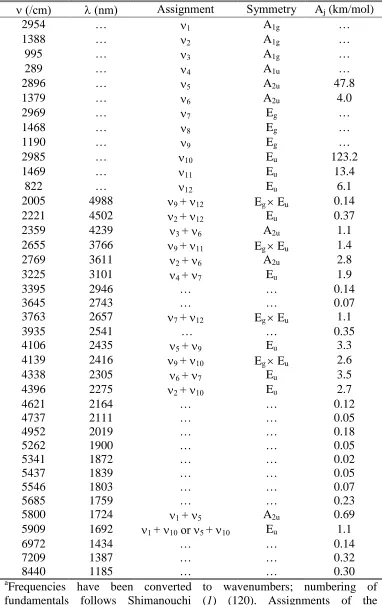
Table 2.1 Fundamentals and observed combination bands of ethane from Figure 2.7.a ...88

Table 3.1: The composition range of recombined components into petroleum fluid base oils. The GOR shows the relative concentration of recombined fluids to the petroleum base. ...152

Table 3.2: Shown are the thin layer stack recipes for the designs discussed. Each row shows the thickness of the thin film for the material shown in the last column. The first column shows the layer number with the first layer being deposited directly onto the substrate and the last layer for that design exposed to air. The second column “MOE Design (nm)” shows the recipe for the fabricated methane MOE. The third column, “Alternate Design (nm) shows a design that was not chosen for fabrication, but rather listed for comparison to the selected design due to the good SEC but very low sensitivity. The fifth column shows the bandpass filter fabricated in this study. The fifth column, ”Uniformity Test Design (nm)”, is an MOE chosen for sharp easy to measure features but difficult to fabricate so that an upper boundary of wavelength fabrication tolerance can be established. ...153

Table 3.3: The results of the MOE fabrication system uniformity test. Twenty MOEs were fabricated on substrates for each of the 6 mm substrates and 25.4 mm substrates. The standard deviation for each peak of the each batch is calculated. The mean position difference for each peak is also calculated for the 25.4 mm substrate to the 6 mm substrate. ...154

Table 3.4: Laboratory validation work for MOC Sensor Series 1, 2, and 3. All measurements presented are acquired at 93.3°C and 40.369 MPa. The reference values are reconstituted with methane to known concentrations with an uncertainty of approximately +/- 0.00005 g/cc methane. Live oil samples labeled LO were run as blind validation. ...155

Table 3.5: Results for the field test of MOC sensors using the methane MOEs. Samples 1-4 are oil samples with reference accuracy of approximately +/- 0.002 g/cc methane to one standard deviation. Samples 5-6 are gas samples with reference accuracy of approximately +/- 0.001 g/cc methane. All samples were run as blind validation. ...156

(12)

xi

fluids to the petroleum base. The design sets for methane and carbon dioxide dual-MOE cores are mutually exclusive. ...216

Table 4.2: Stack designs for MOE dual cores. ...217

(13)

xii

LIST OF FIGURES

Figure 1.1 Shown is an illustration of a generic petroleum fluid phase diagram. The phase envelop is the typical shape of petroleum fluids. The phase envelope separates the single phase fluid region of liquid or gas outside the envelope from the two fluid phase region of liquid and gas inside the envelope. The critical point which lies along the phase envelope separates gas at higher temperature from liquid at lower temperature. The bubble point is defined as the point at which as less dense gas first bubbles from the liquid oil at reservoir temperature.(9) ...28

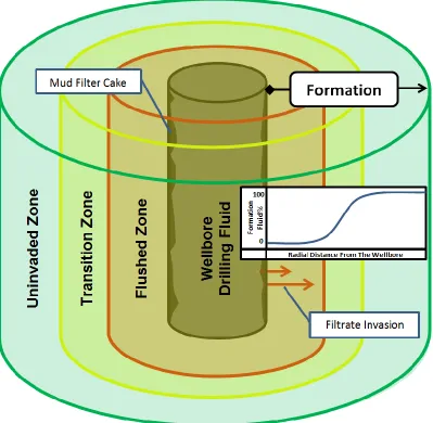
Figure 1.2 Shown is an illustration of a cylindrical section of a fluid saturated formation centered on a wellbore containing drilling fluid filtrate. Filtrate invasion is driven into the formation, displacing the formation fluid in a near wellbore region. The invasion rate is proportional over burden pressure, and inversely proportional to the thickness of the mud filter cake. Filtrate invasion profiles have been modeled by finite element simulation.(50-53) The transition shown by the imbedded graph is a generic illustration of the typical formation fluid profile throughout the three zones which have been described. The imbedded graph is aligned with the radial zones in the illustration grading from 0% formation fluid in the near wellbore region to 100% formation fluid in distal to the wellbore in the uninvaded zone. ...29

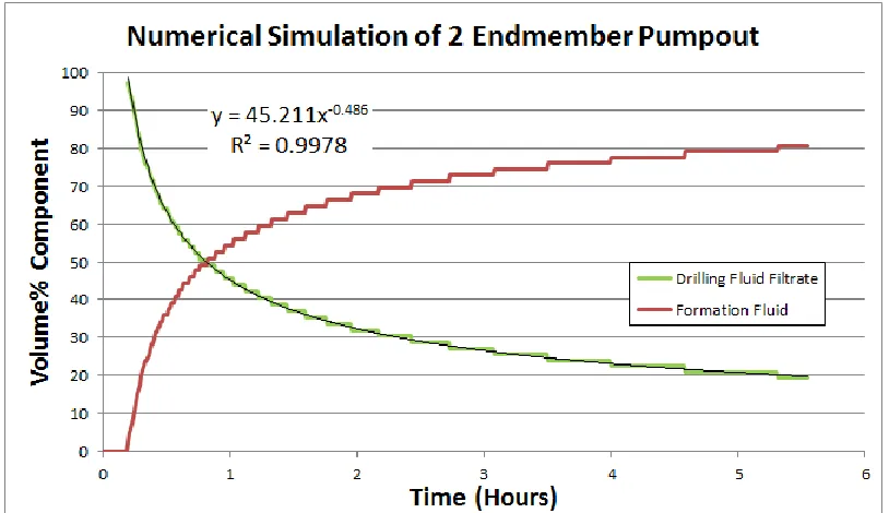
Figure 1.3 A numerical simulation of a formation pumpout assuming a 16 inch radial invasion depth of filtrate with an additional 16 inch radial linear graded convectively mixed transition zone with a formation fluid, homogeneous and isotropic permeability and 0.25 porosity, rate limited by a pumping speed of 40cc/min with a Lamar flow velocity profile. ...30

(14)

xiii

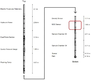
accurately records the fluid density to +/- 0.01 g/cc 95% confidence, with a resolution of 0.001 g/cc. This section also contains a capacitance sensor and resistivity sensor. The MOC sensor is an optical sensor capable of detecting methane and carbon dioxide as the subject of this work. The sample chamber holder switches the fluid from the wellbore exit path into any sample chamber. The spacer contains a series of retractable thermometers for measuring wellbore temperature, but also a shock absorber to minimize impact during descent. The ram is wider than the spacer, and spherical in shape with the intention of preventing sticking on an uneven wellbore surface during decent. ...31

Figure 2.1 Schematic. The top section is used to prepare injections of volatiles. The center section is the main section of the PVTX instrument housed in an oven. The lower right portion of the instrument is used to prepare and inject nonvolatiles and to extract samples for analysis. Valves are labeled v1 to v19; I is a pump driving hydraulic sample injection pumps H3 and SC; Q1 and Q2 are pumps driving hydraulic recirculating pumps H1 and H2, respectively; F is a particulate filter for injected oils; SI is a sample-injection valve; D is a densitometer; PT1 is a pressure and temperature gauge; EC is an oven enclosing the temperature-regulated portion of the instrument; O1 and O2 are fiber-coupled optical cells for FTIR and UV-visible spectroscopy, respectively; C1, C2, CO2, C3, and NGL represent sample loops that can be loaded with volatiles for preparing injections. All Rs represent gas regulators for the respective volatiles, and all Ps represent pressure gauges for the volatiles. See the text for details. ...90

Figure 2.2 Optical cell sketch. The stainless steel cell (A) is constructed to couple to a SMA fiber connector (B). The light is coupled to a 1/8-in. sapphire rod (E) that is held in place with a custom bushing (C) and seal (D). Each sapphire rod extends into the flow path and is set to provide a 1-mm optical pathlength. ...91

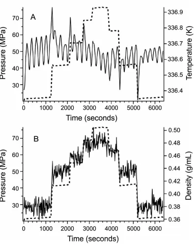
Figure 2.3 Pressure, temperature, and density measurements for a typical isothermal compression/decompression cycle for ethane: (A) measured pressure (dashed line, left axis) during cycle and measured pressure (solid line, right axis). Regular temperature fluctuations result from the reversals of the mixing pumps. Spikes in the instantaneous temperature occur at each step of compression/decompression, but all within approximately 0.5 K of the setpoint. Spectroscopic measurements are made after settling; (B) density (solid line, right axis) during the same cycle as measured by the

in situ densitometer. Correspondence between these measurements and literature are described in the text. ...92

(15)

xiv

Figure 2.5 Ethane absorption spectra in the NIR region between 5040 to 6060 cm-1 (1650 to 1850 nm) under isothermal conditions at 362 K for a range of pressures. Colored curves correspond to the left axis and have been compensated for the density and pathlength changes as a function of pressure and then scaled together for illustrative purposes. The black curve represents the difference between the lowest and highest pressure conditions. Again, in arbitrary units, the zero for this curve is the black horizontal line. Arbitrary scales on the left and right have the same range but different zeros; the black curve has been multiplied by a factor of five for clarity. ...94

Figure 2.6 Ethane spectra respond differently to changes in temperature and pressure. The top curve is the absorption spectrum (corrected for density and pathlength) at a particular temperature and pressure in the strongest part of the NIR spectrum. The colored curves represent changes in absorption in this spectral window when the temperature or pressure vary around this condition. Both difference curves are between the lower and higher density conditions. The red curve represents the change in absorption with pressure, calculated as the difference between a low (21.2 MPa) and high (82.5 MPa) pressure spectrum. The blue curve represents the difference between a high (388 K) and low (337 K) temperature spectrum. The blue and red curves lie on the same arbitrary axis, with the zero difference line shown as a horizontal black line. The colored curves are each multiplied by five to show them on the same axis range as the upper curve. ...95

Figure 2.7 Ethane molar absorption coefficient in the C-H stretching fundamental

absorption region near 3000 cm-1 out to the short-wave NIR. The fundamental absorptions themselves are too strong to be measured in this spectrum because of the relatively long pathlength. All of the stronger bands here have been assigned as either fundamentals (off scale) or combination bands of ethane in Table 2.1. ...96

Figure 2.8 200 parts per million by volume (ppmV) methyl mercaptan (methanethiol) in a balance of methane as a function of pressure at 8.89cm pathlength. ...97

Figure 2.9 A typical live oil spectrum shown from 450 nm in the visible to 5000 nm in the mid infrared acquired at a pressure of 82.76 MPa and 394K 1mm pathlength. Absorbance limit for the visible spectrometer is above 3 abs and for the FTIR spectrometer above 2.5 abs. ...98

(16)

xv

Figure 3.2: Custom band pass filter vs. an ideal top hat baseline offset. The deviation from an ideal reference is compensated by the MOE design. ...158

Figure 3.3: The MOE reference configuration. A regression vector is designed from a spectral library and encoded as the transmission function for an MOE (shown in orange). As light (blue arrow) passes through an unknown sample, represented by the cloud, the resultant light (red arrows) passes through the MOE and onto a detector, whereas a separate path of light is passed through the reference (in green) and onto a detector. ...159

Figure 3.4: Color map of the PLS SEP for beginning wavelengths to ending wavelengths for methane. Dark blue is low SEP better than 5% relative to the methane calibration range, and dark red is higher than 30% SEP relative to the calibration range. ...160

Figure 3.5: Top-down schematic of the ion-assisted e-beam deposition system. ...161

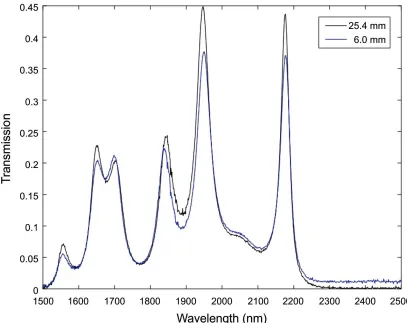
Figure 3.6: Middle MOE transmission of 20 optical elements for a 25.4 mm vs. 6.0 mm double-sided fabrication. ...162

Figure 3.7: Knee-plot of model error vs. number of PLS model levels. The SEP by RMSECV is shown in blue and SEC by root mean square error of calibration (RMSEC) is shown in red. ...163

Figure 3.8: Temperature stability and repeatability of custom bandpass. The leading edge at 1502.6 nm has a temperature stability of 0.0495 +/- 0.0004 nm/°C and trailing edge at 2388.5 nm has a temperature stability of .0374 +/- 0.006 nm/°C. The repeatability of the leading edge is +/- 3.1 nm and trailing edge is +/- 1.4 nm for the batch at the 95% confidence interval. ...164

Figure 3.9: The virtual sensor spectra used for calibration are generated as the vector product of the transmission function for all optical components in the MOC sensor, thereby representing the spectra that the MOC detector would observe. ...165

Figure 3.10: Methane 5 level PLS regression vector for FTIR virtual sensor single beam transmittance. The regression vector is designed to the virtual sensor single beam transmittance calibration set. ...166

(17)

xvi

Figure 3.12: MOE transmission profile for a large (red curve) and small (black curve) regression coefficient design. Note this transmission profile is not convoluted with the custom band pass filter. ...168

Figure 3.13: Fabricated MOE stack compared to the theoretical transmission based on the stack design. The differences in the target design vs the fabricated MOE are due to the re-optimization process. As little stack errors build layer upon layer during the fabrication process, the nonlinear optimization routine uses the in-situ measured optical constants and the transmission profile for the partially fabricated MOE to re-optimize the remaining layers in order to achieve the best SEC performance as opposed to retaining the original transmission shape. ...169

Figure 3.14: Measured vs. predicted methane concentration comparison between theoretical PLS model and MOE design. ...170

Figure 3.15: Temperature analysis results for 200 random seeded designs, using the same random seeds for the single- temperature vs. multitemperature optimizations. ...171

Figure 3.16: Performance for the combined validation study of methane by MOC sensor compared to laboratory gas chromatography analysis. ...172

Figure 4.1: PLS model prediction plot identifying a theoretical PLS calibration error of 0.00478 g/cc (a), and corresponding four-PC regression vector (b). ...219

Figure 4.2: Figure, norm of NAS vs. measured carbon dioxide concentration for the NIR (a) and MIR (b) spectral regions. The range of the MIR NAS indicates~27stronger sensitivity compared to the NIR spectral region. ...220

Figure 4.3: Transmission spectra of the pressure, volume, temperature (PVT) fluid spectra calibration dataset used for carbon dioxide. ...221

Figure 4.4: Carbon dioxide single- and dual-core MOE design results for 500 randomly seeded designs. To help identify viable candidates, MSQ is plotted against SEC (a) and SEC against NNAS (b). The dashed green line plots the PLS limits to serve as a reference point. ...222

Figure 4.5: Dual-core MOE transmission profiles for carbon dioxide (a); optical regression vector based on weighted regression coefficients and the spectra of the optical MOE core pairs (blue circles) and comparison with the single-core optical regression vector (b). The red line of (b) illustrates the reference offset level for positive vs. negative coefficients of the single core as determined by  for a single-core design. ...223

(18)

xvii

Figure 4.7: Methane single- (red triangles) and dual-core (blue circles) MOE design results for2,500 randomly seeded designs plotted vs. the norm of the NAS. The PLS limits (dashed green line) serve as a reference point. ...225

Figure 4.8: Dual MOE core design transmission functions (a) and dual MOE regression vector with PLS regression vector (b). ...226

Figure 4.9: Predicted concentration of carbon dioxide for reference oils run at 62.05 Mpa and 65.5°C based on the theoretical MOC virtual master response. ....227

(19)

1

CHAPTER 1 INTRODUCTION

1.1 THE PETROLEUM INDUSTRY

The petroleum industry is estimated at 4.46 trillion United States dollars (USD)

value as of August 2017, as the composite market cap of 1,618 publically traded

companies tracked worldwide by the Financial Times.(1) This estimation does not

consider private companies and national oil companies (NOCs) such as Saudi Aramco,

and Kuwait Oil Company. The 2016 Oil and gas sector revenues, as tracked for the

largest 45 publically traded petroleum companies of the Fortune Global 500, have a

combined total revenue of 3.3 trillion USD, a number that excludes the NOCs and

smaller independent producers with revenue less than 22 billion USD annually.(2) With

the organization of the petroleum exporting countries (OPEC), accounting for a majority

of the world’s national oil company production, the OPEC market share of 40% (3) can

be used to estimate revenue of 2.2 trillion USD for national oil companies bringing the

global petroleum industry estimate 5.5 trillion USD revenue. The oil industry produced

an average 95 million barrel production of oil per day in 2015, with transportation sector

accounting 60% of the consumption and gas, industrial consumption and chemical

production accounting for the balance (3). During the year 2016 gasoline traded for a

global average of 1.4 USD based on the NasDaq commodity exchange (4) thereby

accounting for about 1.2 trillion USD of annual revenue in 2016 for the oil and gas

(20)

2

chemical sector. Petroleum is in high demand with this demand expected to grow until

2040 as a moderate projection.(3) To meet this demand, approximately 2100 drilling rigs

are in operation for the year 2017 vs 1600 drilling rigs from 2016.(5) Costs for deep

water offshore wells can exceed 1 million USD/ Day with total well costs above 100

million USD/ Day.(6) Two thirds of the wells drilled use formation evaluation services

which includes in-situ formation testing fluid analysis and sampling services. The same

report shows the strongest need for technology improvement, as determined by 278

oilfield operator corporate responses, is improved sensor resolution with 25%, sensor

innovation with 15%, and reliability improvement with 12% as the number one driver,

with no remaining category receiving above %7.(7)

1.2 PETROLEUM FRACTIONS AND COMPOSITION

Petroleum is a geological fluid mixture that can contain of thousands of

hydrocarbon and non-hydrocarbon components.(8-13) The fluid may either be in the

liquid or gas state at reservoir conditions. Hydrocarbon components only contain the

atoms of carbon and hydrogen, where as non-hydrocarbon components may be organics

that contain other atoms known as heteroatoms, or inorganic components. The most

common heteroatoms are nitrogen, sulfur, and oxygen, although phosphorus, and the

transition metals nickel and vanadium, iron and copper, can be found to a lesser extent.

(12,14-15) The carbon dioxide, nitrogen, hydrogen sulfide are the typical inorganic

non-hydrocarbon gas components associated with petroleum.(10,12) Within the petroleum

industry, the carbon number is the common nomenclature for groups of molecular

components with the same number carbon atoms.(8,12) Molecular groups are

(21)

3

molecule. Therefore C1, C2, and C3 are exactly methane, ethane, and propane, but C4

refers to normal butane, and isobutene, C5 refers to all isomers of molecules containing 5

carbon atoms and so on.

Petroleum is formed from the thermogenic cracking of buried detrital biomass, of

primarily plankton sources.(10,16) The buried biomass first fuses under temperature and

pressure, and then at higher temperatures ultimately cleaves by a first order

decomposition reaction forming smaller organic components. The progressive cracking

of organic matter into subsequently smaller compounds leads to a characteristic

exponential decay (log linear) distribution as a function of carbon

number.(8,10,14,17-23) Hydrocarbon components include the hydrocarbon gases methane, ethane, propane

and the isomers of butane and pentane. Hydrocarbon gases are defined as components

that are thermodynamically stable as a pure state in the gas phase at stock tank

conditions, namely 60F (15.5C) and 14.7 psi (1.01 bar).(8-9) Methane is the primary

hydrocarbon gas and at stock tank conditions is usually greater than 70% of the

hydrocarbon gas phase volume, and frequently about 80% to 85%.(9,24-25) Non

hydrocarbon gases commonly found in petroleum are primarily carbon dioxide, nitrogen,

and hydrogen sulfide. Carbon dioxide varies greatly in abundance within petroleum gas

and can typically account for trace concentration to 5% by volume of the produced fluid

stock tank gas phase, but can be a majority of the gas phase reaching 10% to 90%.(9,26)

Nitrogen, when present is usually found in concentration of less than 1% by volume at

stock tank conditions. Hydrogen Sulfide, when present is usually found in concentration

of less than 1% by volume of petroleum at stock tank conditions. Typically, the majority

(22)

4

Components with 6 or more carbon atoms (C6+) are the liquid fraction.(8-9) The

C6+ petroleum fraction is divided into four common sub fractions of hydrocarbons and

non-hydrocarbons. The hydrocarbon fractions include the C6+ saturates fraction and

C6+ aromatics fraction. The non-hydrocarbon fractions include the C6+ resins fraction

and the C6+ asphaltenes fraction. The resins and aromatics fraction increase the

solubility of asphaltenes in solution.(10,27-29) High concentrations of the saturates

fraction, hydrocarbon gas, and especially carbon dioxide, destabilize the asphaltene

fraction and favor asphaltene precipitation. A decrease in pressure also destabilizes the

asphaltene fraction.(28-31) The non-hydrocarbon fractions are characterized by

molecules that contain functional groups with atoms other than hydrogen and carbon and

are known as heteroatoms. The non-hydrocarbon C6+ resins and C6+ asphaltenes

fractions generally contain nitrogen, sulfur and oxygen which give the fractions an

electrically polar charge.(10,32)

Petroleum is generally classified into five reservoir fluid types including black

oils, volatile oils, gas condensates, wet gas, and dry gas. Gas vs oil is defined by phase

behavior with respect to reservoir conditions, with oil as liquid being contained in a

reservoir at a temperature lower than the critical point of the petroleum fluid, and gas

being contained in a reservoir at a temperature higher than the critical point. The liquid

oil will bubble a lower density gas from a denser liquid phase upon the reduction of

pressure. Black oils have a gas to oil ratio (GOR) less than 1,700 scf/bbl and may

further be divided into sub classifications of heavy oils, medium oils and light oils. The

sub classifications of black oils are based on American Petroleum Institute (API) gravity,

(23)

5

oil, as measured at the stock tank conditions of 14.7 psi and 60F. The API gravity is

calculated from the specific gravity by Equation 1.1. For the black oils, the heavy oils

are of API gravity less than 22.5, medium oils are between 22.5 and 30 API gravity, and

light oils are greater than 30 and usually less than 40 API gravity. Volatile oils have a

GOR greater than 1,700 scf/bbl, and typically less than 3500 scf/bbl with an API gravity

typically between 30 and 45. Condensates are gas mixtures that precipitate dew with a

reduction of pressure at reservoir temperature. Condensates are typically of GOR greater

than 3,500 scf/bbl and between 35 and 50 API gravity. No phase segregation occurs for

wet or dry gas as a reduction of pressure from reservoir pressure to stock tank pressure,

however, a wet gas precipitates a dew upon temperature reduction to stock tank

temperature, were as dry gas does not precipitate any liquid upon temperature or pressure

reduction from reservoir conditions to stock tank conditions.(9)

𝐴𝑃𝐼 = 141.5

𝑆𝐺 − 131.5 1.1

1.3 DRILLING

Petroleum wells are drilled with a specialized bit used to grind rock and sediment

into chips called cuttings. The bit is located at the end of a specialized pipe called a drill

string. Specialized sections of the drill string close to the bit known as drill collars can

provide control steering control, drilling measurements, rock formation measurements,

power, and telemetry. The grinding action can be provided either by rotation of the drill

string, or direct hydraulic power to the bit supplied by a drilling fluid. The wells start

with a vertical section of at least a few hundred feet, but may deviate to any angle

including horizontal. Wells may be split into multiple branches known as sidetracks.

(24)

6

been drilled to greater than 7700 meters vertical depth in up ultra-deep water of 3174

meters of water (33), although the deepest wells have been drilled to more than 12,200

depth (34). The thermal and pressure gradients of the wells can routinely provide hostel

pressures and temperatures of 20,000 psi and 400 F respectively, although temperatures

and pressures as high as 35,000 psi and 500 F respectively not uncommon.(35)

1.3.1 Drilling Fluid

The drilling fluid, sometimes called a mud, is a fluid containing a high

concentration of solid clay particles. The drilling fluid circulates through the center of

the drill string pipe, out the bit, and back to surface through the annular space between

the drill string and the well. This drilling fluid, called a mud, has a liquid portion that

may be aqueous, organic, or an emulsified mixture of aqueous and organic components.

The drilling fluid serves multiple purposes. The drilling fluid provides an overbalance

pressure to seal the formation and prevent formation fluid influx. The hydrostatic

pressure provided by the mud also prevents the newly drilled and unprotected wellbore

from collapsing. The drilling fluid lubricates the drill string, and the bit. The drilling

fluid also cools the bit. As the drilling fluid circulates to the surface it carries the

sediment and rock cuttings to the surface.(6,36) Also the drilling fluid is designed to

mitigate the presence of hydrogen sulfide, and carbon dioxide for safety, and to mitigate

corrosion.(37-38) The maximum extent to which a well section may be drilled is

determined by the drilling fluid weight, although other factors may limit the well section

extent. Specifically, the hydrostatic pressure at the top of the section must be high

enough to prevent formation fluid influx, and hence blowouts, while remaining below the

(25)

7

can also cause a blowout. The drilling mud places a hydrostatic pressure on the rock

formation as it is drilled, and maintains that pressure until the section is cemented and

cased.(6)

1.3.2 Invasion

Because the mud is weighted to provide a hydrostatic pressure on the formation

as to keep the formation fluids from invading the wellbore, there is a net driving force for

liquid filtrate to enter the formation. Clay particles which build on the surface of the well

into a filter cake, compresses over time to form a low permeability barrier which prevents

further loss of fluid into the formation.(39) Therefore, as a result of the drilling process

a near wellbore invaded zone of drilling fluid filtrate if formed. Typically this zone

extends from 8 to 32 inches.(40) The organic components of a drilling fluid can be

petroleum distillation fractions such as diesel or mineral oil, or synthetic components

such as olefins, esters, or ketones.(36,41-42) For oil (organic) based mud, OBM, the

filtrate is highly miscible with petroleum formation fluid, and as such there is no

laboratory technique to exclusively separate them without disturbing the inherent

petroleum composition.(43)

The invasion process, as shown in Figure 1.2, has been commonly described as

piston displacement.(39-40,44-48) Piston displacement is the common invasion model

used for simulations, although other models if invasion have been proposed.(49-54)

Figure 1.2 is an illustration showing a cylindrical section of a generic, fluid containing

formation, centered on a wellbore. The mud filtrate invasion displaces the formation

fluid, much like a plug, from the near wellbore region. As shown in Figure 1.2, three

(26)

8

transition zone comprising an composition intermediate to that of the filtrate and

formation fluid; and 3) The uninvaded zone containing the native formation fluid.

Together the flushed zone and transition zone comprise an invaded zone. All three zones

are observed by formation probing sensors including resistivity sensors, nuclear sensors,

acoustic sensors, and NMR sensors.(39)

1.3.3 Formation Evaluation

The hydrostatic mud column pressure is specifically designed to contain a

formation fluid within the rock formation.(6,36) Therefore, evidence of petroleum within

a zone is suppressed and not obvious without closer inspection of the formation. It is

surprisingly easy to drill through a potential petroleum reservoir, and never determine its

existence, only to discover the bypassed pay decades later upon re-evaluation of the

formation log data.(55) In fact, the metadata results for the search of “bypassed pay” in

the OnePetro petroleum industry database operated by the Society of Petroleum

Engineers returned 1255 articles, suggesting that the occurrence of “bypassed pay” is

painfully common.(56) To find a petroleum reservoir within a well, the well must be

evaluated by sensors specifically for the presence, nature and quality of liquid or gas

petroleum. Also, the formation is evaluated for rock properties indicative of reservoir

quality. Methods of evaluation include wireline and or logging while drilling sensing,

surface data logging, fluid and core sample evaluation, and well testing. The formation

evaluation is conducted on the open hole prior to casing and cementing a well

section.(6,57-58)

Surface data logging, attempts to measure the change in drilling fluid properties

(27)

9

cuttings are carried to the surface and depressurize, the formation fluid contained within

the cuttings evolves into the drilling fluid as mud gas.(59-60) Mud gas is analyzed at the

surface on the drilling rig platform, by gas chromatography and spectroscopic equipment.

Mud gas analysis provides a qualitative gas distribution but not reservoir fluid

concentration.(61) However, the gas distribution and isotopic content can indicate the

presence and nature of formation fluids. Also, the evaluation of the rock cuttings can

also provide some formation properties.(59-60) Unfortunately the exact location of a

petroleum occurrence is not known with high resolution as the cuttings and fluid churn in

transit to the surface.(6,62)

Wireline and Logging While Drilling (LWD) sensor evaluation can provide a

more accurate location of formation and fluid properties along the wellbore.(6, 57-68)

For a wireline evaluation, sensors are lowered into the well along a wireline cable that

provides telemetry and power. The sensors probe the formation from a distance. The

electrical wireline cable provides direct kilowatt range power with up to megabit speed

telemetry for in-situ sensors.(6,58,63) LWD logging places the sensors in specialized

drill pipe sections called collars, which are just behind the drill bit, as part of the bottom

hole assembly (BHA).(6,58) Although wired pipe for LWD telemetry and power does

exist, it is far more common for those sensors to be powered by battery or generated

power from hydraulic drilling, with surface telemetry provided by mud pulses at about 20

bits per second.(6,64) The conventional wireline and LWD sensors look into the

formation using electromagnetic technology, nuclear physics technology, acoustic

technology, and magnetic resonance imaging technology. The conventional logging

(28)

10

unfortunately convoluted. To provide pure rock and fluid information, the formation fluid

responses and rock responses must not only deconvoluted, but also the effects of the near

wellbore drilling fluid filtrate invasion, and the wellbore drilling fluid influence

subtracted from the logging responses.(58) None the less, in combination with surface

data logging, the information provided by conventional wireline logging can identify

zones of interest for well testing and sampling.(6,57,61)

Well testing is the only logging technology that provides conclusive evidence for

the presence of petroleum deposits within a reservoir zone and the dynamic production

potential of that petroleum.(6) Additionally, the formation fluid properties are provided

in real time which is critical information for safely addressing issues encountered during

well construction.(6,65-66) Well testing includes wireline and LWD formation testing,

and drill stem well testing. In well testing, fluid is withdrawn from the formation and

analyzed separate from the rock formation and well bore drilling fluid. Formation

pressure and production rates are measured as a function of pressure.(6,58,65-66)

A drill stem test produces fluid to surface through specialized pipe or tubing.

Drill stem testing places a temporary production apparatus in a well to produce large

quantities of petroleum reservoir fluid to the surface. At a surface a gas separator

removes the dissolved gas from the liquid oil in a controlled depressurization. The

production rate of oil and gas from a reservoir section is monitored at surface.(6,8) The

liquid oil and flashed gas are sampled separately and analyzed in a laboratory.(8) The test

is usually conducted for days to weeks at considerable expense, but conclusively provides

production potential of a reservoir section, reservoir extent, rock permeability, formation

(29)

11

however, is an average of the produced zone which can span multiple compartments and

any compositional grading that often occurs within a reservoir section is not

preserved.(10,30,65) Unfortunately, the fluid recovered at surface is depressurized and

phase segregated, which can alter the fluid properties, especially with respect to

asphaltene precipitation.(10,30,65,69) The cost is substantial and fluid disposal is of

great concern; hence well testing is not always practical, especially in deep wells, highly

gas charged systems and unconsolidated formations.(67,70-71)

In many cases, drill stem well testing has given way to formation testing which

extends a rubber pad against the formation to make hydraulic contact, measure the

formation pressure, and withdraw fluid using a mechanical pump. The fluid can be

sampled under pressure and returned to surface using a pressure compensating

chamber.(67-68,70) Rock cores can be cut either with a specialized drill bit on the drill

string, or a wireline device which is often run with the formation testing equipment. The

cores can be tested in a laboratory for mechanical rock properties, and fluids withdrawn

and analyzed.(6,36)

1.3.4 Casing and Completions

Each section of a well is cased with a metal pipe to provide fluid isolation and

cemented to provide reinforced well strength and bonding of the casing with the

formation. A well section is usually immediately cased and cemented after formation

evaluation both for safety reasons, and to meet the drilling schedule. Each subsequent

section is drilled with a smaller bit, forming a smaller wellbore. The casing is lowered

into the well and either hung into position as a liner, or from surface as a pipe casing.

(30)

12

casing with a displacement fluid. The casing and cement are selected based on pressure,

environmental and chemical considerations with corrosion and gas content of primary

concern, and hence early fluid analysis is important. After the well has been drilled to the

terminal depth, the well is either cemented and abandoned if purely an exploration well,

or completed if a production well. A well may be temporarily decommissioned if to be

completed and produced at a later date.(6)

To complete the well, explosive charges are lowered into position and discharged,

in the presence of a completion fluid, to perforate the casing and cementing within an

identified production zone. A completion string which may consist of packers and

production tubulars can be lowered into the well to produce from multiple reservoirs

which can be commingled and separate tubulars to zones which may not be commingled.

Production may also take place directly through suitable casing if separate production

strings are not necessary. The completion design is primarily dependent on the reservoir

pressure as well as fluid compatibility. High quality fluid analysis is required to

understand which zones may be commingled. The fluid analysis results regarding the

corrosive nature of the production fluid is a primary concern in selecting completion

designs. The top side facilities, which separate the gas from oil, must be designed for the

proper gas to oil (GOR) as based on the fluid analysis. Additionally, the top side

facilities must also be designed specifically for the chemical corrosiveness of the

production fluid, including scrubbers to prepare the fluid for transport.(6)

1.4 FORMATION TESTING AND SAMPLING

Wireline or LWD formation testing provides petroleum asset evaluation and risk

(31)

13

samples, acquired in the oil well at the reservoir, are a primary means to provide the fluid

properties necessary to simulate production strategies, design completions, design large

capital investment surface facilities, anticipate any flow assurance production issues and

associated operational expenses, and ultimately make the financial decision as to whether

an asset should be developed.(65-66,75) However, the utility of the samples acquired is

only discovered after laboratory analysis. After a delay of transport, the laboratory

analysis often takes weeks to months. Unfortunately, as formation testing is often the last

activity prior to casing and cementing a zone, only one opportunity is available to acquire

these open hole samples, and that opportunity is not afforded the benefit of a second

chance to mitigate poorly acquired samples.(66,73-74)

Accurate compositional measurements of a reservoir petroleum fluid is necessary

to ensure a well is safely drilled, to identify a new discovery, to evaluate the production

potential and value of that discovery, to optimize the capital investment required to the

produce petroleum, and to design a field management system for multiple reservoirs in a

field.(66) There are three primary methods are used to obtain chemical information of a

petroleum fluid contained in a reservoir, mud gas analysis, drill stem tests, and bottom

hole sampling by formation testing. Mud gas analysis is qualitative, and drill stem tests

are often unfeasible.(61,67,69,75) Bottom hole sampling acquires samples directly from

a reservoir with a device lowered along the electrical wireline cable. The device has

pumps designed to extract petroleum from a precise location along the wellbore and place

that sample into a pressurized container which is then sent to a laboratory for

analysis.(8,65-66) Typically on a single wireline sampling run, only 3 to 9, 1000 ml

(32)

14

samples can be collected.(76-77) Based on 10 case studies, 64 samples, with 16 wells and

117 pressure tests for 3 wells, an average formation tester sampling run takes 14.1 hours

for an average 4 samples per well and average pressure test takes 0.36 hours for an

average 39 pressure tests per well.(78-87) Therefore the average formation test pressure

and sampling run, including trip and set time, takes 70.4 hours or almost 3 days. To

acquire 3, 6, and 9 samples on a formation testing run it would take 56, 99 and 141 hours

on average respectively by those statistics. LWD formation testing and sampling

operationally has a similar duration to that of wireline formation testing with estimates of

4 to 7 days, however, LWD formation testers must stay in hole typically from 120 to 396

hours (5 to 16.5 days) for the entire drilling of a well section.(88) It is clear that

formation testing fluid analysis sensors must operate days and survive weeks without

service in harsh environment conditions.

The laboratory analysis of fluids can be performed in as little as 3 weeks but can

also take months, and the transport and a lead time can be weeks to months before sample

analysis can even begin.(73,89) Because samples can be taken at multiple locations

along a single reservoir, the samples are more representative of the reservoir geometry

than with mud gas analysis, or drill stem test samples.(60-61,65) If the samples are kept

above reservoir pressure, the samples are not irreversibly altered. Usually, by the time a

laboratory analysis is performed, the well section from which samples were acquired, has

been shut in cased and cemented, and often, the drilling rig moved to another location.

The laboratory analysis reveals the quality of the sample and hence their

usefulness.(73-74) Unfortunately, as formation testing is often the last activity prior to casing and

(33)

15

opportunity is not afforded the benefit of a laboratory analysis to mitigate poorly acquired

samples, or if those samples were not acquired from the best locations. Therefore some

level of analysis is required in real time to assess the suitability and utility of samples

prior to acquisition downhole. That fluid analysis may also be used to augment the

laboratory data acquired from the samples at sparse locations.(90-91) For this reason,

both physical and chemical fluid property sensors exist in formation testers. Fluid

temperature and pressure, resistivity, capacitance, density, viscosity, bubble point,

compressibility, index of refraction, speed of sound, and compositional sensors are

routinely employed to monitor the properties of fluids during a formation

pumpout.(66,72,76-77) A formation pumpout is the process of mechanically

withdrawing large volumes of fluid from the formation with a formation tester in order to

flush the near wellbore region clean from invasion of drilling fluid filtrate. Usually

between 100 L and 600 L are withdrawn. Figure 1.3 shows a simulation of the fluid

withdrawn from formation during a two endmember pumpout. Multi-endmember

pumpouts are possible if the fluid is withdrawn from a transition zone containing oil and

water, or if the filtrate invasion is an emulsion of oil and water. The two endmember

pumpout considered here is specifically for petroleum based drilling fluid filtrate and

miscible oil based drilling fluid filtrate invasion. The formation fluid grades

monotonically asymptotically from high contamination at early time lower contamination

at later time after an initial breakthrough of formation fluid.

Figure 1.4 shows a diagram of a formation tester, containing the Multivariate

Optical Computing (MOC) sensor, the topic of this study. From top to bottom, the

(34)

16

high voltage 60 Hz alternating current (880 V) to low voltage 60 Hz alternating current

220 V and 20 V direct current. The telemetry sub sends up to 1.2 Mbit/s, and receives

200 Kbit/s with ASDL protocol. The hydraulic power section converts electrical power

to hydraulic power to be used throughout the formation tester for mechanical action. The

dual probe section hydraulically sets up to two donut shaped pads against the formation

like suction cups with 4,000 psi of pressure, balanced opposite by two hydraulic rams.

The probe section also contains a Pressure Volume Temperature (PVT) test cylinder to

monitor the bubble point and compressibility of the fluid withdrawn. The quartz gauge

section accurately reads the pressure of the fluid to +/- 0.1 psi. The flushing pump

section contains a hydraulically powered reciprocating pump with speeds operational

between 2 ml/s and 40 ml/s. The pump withdraws fluid from the formation through the

probe into through the tool sections and with exit to the wellbore through the last sample

chamber section. The densitometer section accurately records the fluid density to +/-

0.01 g/cc, with a precision of 0.001 g/cc. This section also contains a capacitance sensor

and resistivity sensor. The MOC sensor is an optical sensor capable of detecting methane

and carbon dioxide as the subject of this work. The sample chamber holder switches the

fluid from the wellbore exit path into any sample chamber. Up to 5 sample chamber

sections may be stacked, although 1 to 3 are most common due to weight and length

constraints. The spacer contains a series of retractable thermometers for measuring

wellbore temperature, but also a shock absorber to minimize impact during descent. The

ram is wider than the spacer, and spherical in shape with the intention of preventing

sticking on an uneven wellbore surface during decent. The tool sections can be

(35)

17

and ram section at the bottom. The hydraulic power section must be co-located with the

probe section opposite of the flushing pump. The direction of pumping may either be up

or down. The probe section starts the formation flow line and the sample chamber

sections must terminate the formation flow line.

Three critical questions define the success of any open hole sampling program.

Specifically: Where to sample?; When to sample?; and How to sample?(92-93) Samples

must be gathered from the best locations along the wellbore such that fluid trends can be

adequately defined. Reservoir fluids must be sampled at the optimal time during the

formation fluid cleanup pumpout at a point for which the contamination is sufficiently

low as to achieve the goals of sampling. Lastly, the samples must be acquired in such a

way as to ensure they are representative aliquots of the formation fluid, and are

maintained as such in transit from the down hole reservoir to the laboratory.(92)

1.4.1 Where to Sample?

Reservoir compartmentalization and fluid column compositional grading within a

reservoir compartment are the two primary defining factors in assessment of sampling

location.(66,72,90-91,94-99) However, it is the fluid analysis from the samples that will

ultimately confirm compartmentalization and compositional grading.(73,94) Therefore,

it is generally desirable to obtain at least one sample from every reservoir compartment,

and up to three samples from reservoirs which exhibit sufficient compositional grading.

(73,94,100) Conventional wireline log data and formation pressure test data can provide

some compartment information, but little compositional grading information.(94,101)

Fluid properties, including methane carbon dioxide and asphaltene concentration, provide

(36)

18

grading.(66,73,90-91,94-99,101) Significant advancement has been made toward using

downhole fluid analysis data for the purpose of determining sampling location and for

augmenting laboratory sample analysis for final compartmentalization and compositional

grading assessment. Compartmentalization and compositional grading assessment has

been assigned geochemically, statistically, and by thermodynamic principals governed by

cubic equations of state utilizing fluid composition as determined in laboratory studies

and in situ on formation testers.(61,90,94,102-105)

1.4.2 When to Sample?

Samples need to be of sufficient quality to be representative of reservoir fluid

properties. Those samples must be acquired with sufficiently low filtrate invasion

contamination. In acquiring a bottom hole sample it is the goal to collect a sample with

sufficiently low contamination in as short a time as is possible. Multiple sensors for

down hole fluid sensors exist to assess contamination level, however, including methane

concentration and GOR. It is desirable to acquire a sample as soon as it can be

determined with certainty that the contamination is below a threshold required for the

series of laboratory analysis.(25,72,106) Generally, 5% contamination is sufficiently

low contamination for most medium and light oil analysis although 10% to 15% can be

acceptable for some applications.(73,107-108) Volatile oils and condensates phase

envelop is highly influenced by slight contamination and as such less than 3% to 1%

contamination respectively is often desirable.(66,73,107)

Various schemes have been proposed for real time downhole contamination

assessment including, trend fitting (72), endmember fingerprinting (94), and equation of

(37)

19

and ubiquitously. Equation of state methods have required more, high quality input than

is generally available downhole. To date the most common comercial means of real time

contamination assessment is asymptotic trend fitting as shown in Equation 1.2.

(65,93,109) Trend fitting relies on two basic assumptions: 1) That as the instantaneous

pumpout fluid, monotonically grades with volume pumped, from filtrate to formation

fluid, a pure formation fluid is asymptotically approached, and 2) that the pumpout

gradation follows a strict analytical form that may be sufficiently fit as to determine the

asymptote endmembers.(53,109-110) Equation 1.2 shows an asymptotic equation

derived by Hammond(109) for a hemispherical formation tester probe in a homogeneous

isotropic reservoir rock with respect to permeability and porosity. Other equations have

been derived for anisotropic media and other probe configurations.(111-112) For

Equation 1.2 the values SM, SA, and SS are the signals, at the monitor time, asymptote at

infinite time and start time respectively. The volume, V, at start time is not zero, but

rather the volume required to pump in order to clear the flushed zone and first observe

filtrate at the formation testing sensor. The value of 2/3 was derived for a circular probe

of negligible size compared to the wellbore radius, and  is constant dependent on the

formation and fluid properties such that the denominator of Equation 1.2 at the start time

is unity. For trend fitting, a single sensor parameter, linear with contamination, such as

density, methane concentration, asphaltene concentration is required.(113-114)

Contamination is calculated as the percentage of the monitor signal value to asymptote

value difference relative to the starting value asymptote difference shown in Equation 1.3

(38)

20

state, or statistical methods of contamination estimation, accurate, high resolution fluid

measurements with respect to fluid contrast are required.(102,115-116)

𝑆_𝑀 = 𝑆_𝐴+𝑆𝑆− 𝑆𝐴

𝛾𝑉23 1.2

𝐶% =⌊𝑆𝑀− 𝑆𝐴⌋

⌈𝑆_𝑆− 𝑆_𝐴⌉ × 100 1.3

Often the starting value for the monitor signal is not observed and is extrapolated

with some uncertainty. Therefore a third assumption is often imposed, that the starting

monitor value for mud filtrate properties is known. Such is the case with methane and

asphaltenes that are assumed to be zero concentration at pumpout start. Because mud

filtrate depressurizes at the surface, any filtrate which permeates into the formation

ideally contains no methane. Also any asphaltenes that do contaminate the drilling mud,

usually flocculate and hence do not enter the formation but rather cling to the mud cake

on the wellbore surface. Usually either methane or asphaltenes can provide a good

contrast for asymptotic fitting. Petroleum samples with high methane have low

asphaltene concentrations and samples with high asphaltene concentration have low

methane concentration. Therefore methane and asphaltene concentrations are primary

signals for trend fitting. Also, asphaltene gradient, and GOR gradients as a function of

reservoir depth can constrain the ending asymptote for a pumpout, with methane and

carbon dioxide accounting for a majority of the GOR gas.(25,53,72-73,75,106)

1.4.3 How to Sample?

For a sample to be useful in petroleum asset assessment, it must be representative

of the reservoir fluid from which it was aliquoted.(73) Of concern are phase changes

(39)

21

from a bulk fluid.(8) Fluid chemical measurements can provide information about

potential sample fractionation issues while sampling.(66,91,94-95,97) For gas

condensates, it is very common to fractionate a liquid portion from a bulk gas. However,

fractionation of light components relative to heavy components can naturally take due to

differences in mobility, not unlike with the effect of chromatography.(10,25,117-118)

Therefore to ensure a sample is not fractionated as withdrawn from the formation,

methane can be a useful fluid component to monitor.(93) Also, the caustic and reactive

nature of the near wellbore drilling fluid filtrate can fractionate acetic components of a

petroleum sample.(37-38,73) Therefore acetic components of the petroleum fluid such as

carbon dioxide may also be useful to monitor in order to ensure a representative fluid

sample.

It is desirable that the sample be acquired with enough pressure as to ensure

preservation of single phase with regards to a gas/ liquid phase envelop and asphaltene

phase envelop.(30,119) Pressure, preservation of samples receives the greatest amount

of attention with regards to fractionation issues. The asphaltene phase envelop is

complicated with pressure effects, temperature effects, and compositional effects.(11) It

has been shown, that once asphaltenes precipitate from solution, it is not always

favorable for them to attain their reservoir state even when the sample is reintroduced to

reservoir temperature and pressure.(27-28,31,119-120) Also if precipitation of

asphaltenes occurs in the reservoir, an unrepresentative sample may be acquired devoid

of those asphaltene species.(31,119) Therefore it is important to ensure the asphaltenes

(40)

22

1.5 Laboratory Analytical Techniques

After acquired, open hole samples are brought to surface, samples that are not

acquired in Department of Transportation (DOT) certified sample containers are

transferred into certified shipping sample cylinders. This process dictates a single phase

transfer above reservoir temperature and pressure.(77,100,119,122-123) Although not

prevalent, during the transfer, some sample may be aliquoted and analyzed at the well

site.(73,123-125) Wellsite analysis is usually limited to a volumetric flash in which the

sample is immediately lowered from reservoir temperature and pressure to stock tank

temperature and pressure. The gas and liquid phases immediately separate and the

volumes are measured. The ratio of gas to liquid is reported as the GOR. A subsample

of the gas fraction is usually measured in a gas chromatograph with a thermal

conductivity detector (GC-TCD) composition, and a liquid subsample is measured by gas

chromatography with a flame ionization detector (GC-FID) for composition. Up to the

C10 components, individual species may or may not be reported, but above C10

individual components are rarely reported. Carbon numbers are reported as a plus

fraction of usually 10 to 30. A stock tank condition density is usually measured for the

liquid fraction. The gas and liquid compositions are re-combined mathematically using

the molecular weight estimated from the compositional analysis, density of the liquid

fraction and the measured flashed volume, as the reservoir fluid

composition.(8,12,73,123,125-128)

The DOT certified shipping sample cylinder is sent to a laboratory for analysis. It

is standard for the DOT certified cylinder to contain a mixing ball to aid in sample

(41)

23

sample was in an airplane cargo hold, the sample may have been exposed to temperatures

well below freezing. Otherwise the samples were at least exposed to the environmental

temperatures during transit, which may also be below freezing. In some circumstances,

the temperature of exposure may lower the pressure in the cylinder below the cylinder

compensation system’s ability to keep the sample above a multiphase envelope. The

sample is therefore restored to reservoir conditions, over the course of 1 to 3 days, but

sometimes up to 1 week. Standard restoration consists of heating the sample back to

reservoir temperature, maintaining pressure at reservoir pressure, and mixing the sample

cylinder by rocking it back and forth with the mixing ball providing

agitation.(8,69,77,124) Once recombined, the flash and compositional measurements are

made as described above. However, in the laboratory, is also standard laboratory practice

to measure the molecular weight of the liquid fraction by freezing point depression as

opposed to estimation by composition. Also it is standard practice to measure the density

of the gas fraction in order to calculate the molecular weight of the gas fraction. The

density of the liquid fraction is measured as before. Chemical analysis for geochemistry,

oil fingerprinting and biomarker analysis such as two dimensional Gas Chromatography

(GC X GC), gas chromatography with a mass spectrometry detector (GC-MS), Fourier

transform ion cyclotron resonance mass spectrometry (FT-ICR MS), and Isotope Ratio

Mass Spectrometry (IRMS).(10,12,129)

To determine the composition and physical properties of the pure reservoir fluid,

acquired with formation testers, it is necessary to provide a good estimate of the

concentration of drilling fluid filtrate, and back out that effect.(130-131) The drilling