Using Entropy Working Correlation Matrix in Generalized Estimating Equation for Stock Price Change Model
SerpilKılıç (Faculty of Arts and Sciences, Department of Statistics, Yıldız Technical University, Davutpasa Campus, 34220, Esenler, İstanbul)
Ahmet Mete Çilingirtürk (Faculty of Economics and Administrative Sciences, Marmara University, Bahçelievler Campus, 34180, Bahçelievler, İstanbul)
Author (s)
SerpilKılıç Res. Assist., Faculty of Arts and
Sciences, Department of Statistics,
Yıldız Technical University,
Davutpasa Campus, 34220, Esenler,
İstanbul.
E-mail: [email protected]
Ahmet Mete Çilingirtürk Prof. Dr., Faculty of Economics and
Administrative Sciences, Marmara
University, Bahçelievler Campus,
34180, Bahçelievler, İstanbul. E-mail: [email protected]
Using Entropy Working Correlation Matrix in Generalized Estimating Equation for Stock Price Change Model
Abstract
Longitudinal studies involving binary responses are widely applied in medical, health and economic science research, have focused increasingly on how various independent variables affect responses over time. These studies involve repeated observations on a subject and thus correlation within each subject is expected. Correct inferences can only be obtained by taking into account the correct specification of within-subject correlation structure between repeated observations. In recent years, non-normal longitudinal data is analyzed by Generalized Estimating Equations (GEE) method. Goodness-of-fit statistics have been suggested for selecting an appropriate working correlation structure in GEE with longitudinal binary data. The purpose of this article to provide an overview of the GEE approach for analyzing correlated binary data and to choose the structure of the correlation matrix between repeated observations for model comparison, using data from Istanbul Stock Exchange (ISE) to increase on the return.
Keywords: Working Correlation Structures; Generalized Estimating Equations; Longitudinal Binary Data; Entropy
JEL Codes: C33, G00
Introduction
Generalized estimating equations (GEE) approach which extends generalized linear models is a very popular for the situation of correlated data obtained longitudinal studies. Although GEE models can be used for
each time point. (Hedeker and Gibbons, 2006, 135). This approach is complex to interpret and implement from classical analysis approach. Despite the many benefits of classical analysis, it has some constraints. These are: (1) it does not model the mean response changes across time on each subject; (2) it has some assumptions about the variance-covariance matrix. For example; in the classical regression model, a single observation of the response variable is considered as the observational unit. Therefore, the statistical modeling assumes independence between observations (Lee et al., 2007, 188). But the assumption of independence is not usually used in longitudinal studies, because the relationship between repeated observations over time on the same subject can be correlated; (3) it does not consider about the structure of dependence between repeated observations obtained from the same subject. For these reasons, the classical approaches are insufficient.
The structure of correlation is important to produce efficiency (i.e., statistical power) in the estimation of the regression parameter. However, the loss of efficiency is lessened as the number of subjects gets large. If the correlation data is correctly identified, the inferences about hypothesis tests and confidence intervals will be valid and correct.
In this study, we consider to correlated binary data and compare several criteria that can be obtained the final selection of
working correlation structure. Generalized Estimating Equations A review of GEE method GEE models are used for analyzing longitudinal binary studies involve binary responses for each subject and a set of covariates varying with or without time. Consider a longitudinal binary data set comprising (Xit,Yit) for i=1,…,n; t=1,…,ni.
For the ith subject, there are ni repeated
binary response variables. Define a nix1
binary response vector as Yi=(Yi1,…,Yini)'
and a nixp covariate matrix as
Xi=(Xi1,…,Xini)' with a p-dimensional
covariate vector Xit. The binary response
variable Yit=1 at time t, if the subject i has
response 1, success and Yit=0 if otherwise.
It is assumed that ni=m for all i and N=mn
(Lin et al., 2008, 4428).
The most important problem in this method is to determine the (co)variance structure. Even if the covariance structure has been misspecified in longitudinal studies, GEE method yields asymptotically normal and consistent for estimated parameters. GEE specifications are similar to generalized linear model (GLM), but those of GLM with one addition are comprised by GEE approach. There are three specifications in this model. First, the linear predictor is given as
……….(1)
The common choices for link function are identity, logit, and log for continuous, binary and count data, respectively. The variance is described as a function of the mean,
………..(3)
where υ(μit) is a variance function and ϕ is a
scale or distribution parameter. When each subject is measured at all m time points, the working correlation matrix of the repeated observations is of size mxm. If a subject has been measured at nitimepoints (ni<m), each
subject’s correlation matrix Ri will be of
size nixni. α is a vector of association
parameters which are assumed to be the same for all subjects. (Hedeker and Gibbons, 2006, 135)
Working Correlation Structures
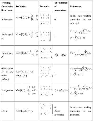
There are some possible correlation structures to be appropriate to use in GEE. These structures are independent, exchangeable, autoregressive, m-dependent and unstructured. The most commonly used working correlation structures and estimators are given in the Table 1.
If data is balanced and there are clusters with small number of observations, the unstructured correlation matrix is recommended. An exchangeable correlation matrix may be most appropriate for datasets with clustered observations, which may not have a logical ordering at observations within a cluster. When the observations have been mistimed, it may be appropriate to regard a model where the M-dependent
or autoregressive correlation is a function of the time between observations. Any estimation of α is not performed for both the independence and fixed working correlation structures (Horton and Lipsitz, 1999, 161). This paper presents the use of entropy for working correlation matrix, which supports an unstructured dependence within the time points. Although the word “entropy” originated in the literature of thermodynamics, its usage has penetrated almost all disciplines due to its association with the concept of information as envisaged by Claude Shannon.
If the probabilities can be used rather than raw results, entropy can be calculated for one variable and can also be used for researching dependence between two or more variables. Due to this future of entropy, it could be a possible alternative for correlation coefficient. Because of the importance of working correlation matrix in GEE, it is crucial to use different working correlation structure in order to obtain efficient results. Therefore, entropy matrix could be the possible alternative for common working correlation matrix. The entropy and entropy correlation coefficient( ) formulations are given in Equation 4-8.
………….(4)
………(6)
..……(7)
…..(8)
GEE Estimation
The working covariance matrix for Yi
equals ….….…(9)
where Ai is mxm diagonal matrix with V(μit)
as the tth diagonal element. ϕ is an overdispersion parameter that can be
estimated as
follows:
.(10)
where N is the total number of observations and p is the number of regression parameters. The square root of the overdispersion parameter is called the scale parameter.
The GEE estimator of β is the solution
of ....(11)
where Di is the matrix of derivatives
………(12)
Iterative process for GEE’s is given the following:
1.Start with Ri=independent (i.e., identity)
and ϕ =1: estimate β.
2.Use estimates to calculated fitted
values:
3. Residuals:
4. These are used to estimate Ai, Ri and
5. Then the GEE’s are solved again to obtain improved estimates of β.
…….(13) 6. Between step 2 and 5 are repeated to
converge to a value of β (Kılıç and Çilingirtürk, 2011, 327).
Model Selection and Goodness of Fit Tests
This paper examines three model selection criteria which are Marginal R2, QIC and QICU estimates.
Repeated observations are correlated over time points, therefore residuals are not independent. R2 in the ordinary least squares method cannot be used for GEE directly. An extension of R2 statistics in GLM is called as Marginal R2 for GEE (Zheng, 2000, 1268). It can be calculated as shown below.
One of the goodness-of-fit statistics, Akaike’s Information Criterion (AIC), can be used for comparing competitive models. But this criteria could not be used for GEE method. Because GEE is not a likelihood-based method. In this reason, Pan (2001) introduced a selection method which named as Ouasilikelihood under the Independence Model Criterion (QIC). QIC is similar to AIC. The formulas AIC and
QIC are given as
follows: ………(15)
where L is the log likelihood and p is the dimension of β.
… ….(16)
Is quasi likelihood computed using R, Ω ̂_I is the inverse of the variance matrix by fitting an independence model and is modified sandwich estimate of variance from the model with R in Equation 16.
When approximates p, Pan (2001) also proposed QICU which could be
useful in variable selection, but it is not used for model comparison. QICU’s formula
is given in Equation 17 (Hardin and Hilbe, 2003,
139). …(17)
Marginal R2, QIC and QICU are the criteria
of the evaluation of choosing the best model.
In this process, the model with lower value of QIC and QICU and higher value of
Marginal R2 should be taken into account. These criteria are obtained by special macro software in the SAS 9.2 program (support.sas.com/resources/papers/proceedi ngs09/251-2009.pdf, 2011, 5).
Stock Price Change Model
The significance and purpose of this study
prices and volume. Technical analysts do not attempt to measure a security's intrinsic value but instead use stock charts to identify patterns and trends that may suggest what a stock will do in the future” (http://www.investopedia.com/ask/answers/ 131.asp, 2011).
Data Sources
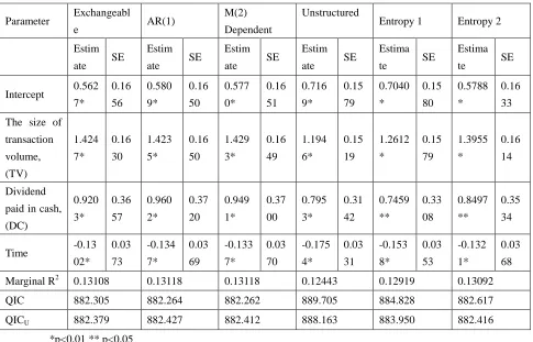
Using 100 transactions data chosen ISE between 2008/12 and 2010/12 quarterly, we estimate parameter estimates and the corresponding standard errors under exchangeable, AR(1), M(2) dependent, unstructured and entropy correlation structures via GEE method. We compare the criteria for choosing between these structures. In this study, response variable is stock price. According to the technical analysis, it is coded 1 if it increases according to the previous 3-month period, otherwise 0. Covariate variables are transaction volume, stock dividend, cash dividend, increase of capital, price index, exchange rate of dollar, Nomenclature Generale des Activites Economiques dans I'Union Europeenne, NACE, (General Name for Economic Activities in the European Union) Codes and time. Transaction volume and dividend paid in cash are coded 1 if it increases according to the previous 3-month period, otherwise 0. The effects of NACE, increase of capital and stock dividend of these factors on stock return are not statistically significant. We take the transaction volume and dividend paid in cash as the covariate variables.
Findings and Results
Let μit denote the mean, the probability of
increasing stock prices for i=1,…,100 stocks and t=3 (baseline), 6, 9, 12, 15, 18, 21, 24 months. logit link function for binary responses can be shown as follows:
…(18)
where β0, β1, β2, β3 are the regression
is preferred. Conclusions
We have discussed selecting the working correlation structure in GEE with longitudinal binary response. An application of longitudinal studies to data on stock price is used as an example. GEE is relatively new method for the analysis of longitudinal studies on stock price. GEE method yields the estimates of regression coefficients and their variances from different correlation structures that can be sensitivity to incorrect specification. will be estimated asymptotically normal and consistently, even when the working correlation structure is misspecified. The choice of Ri will
influence the efficiency for estimates of parameters and variances. It is more efficient to use Ri that is chosen correct
specification. For this study, the results of the correlation structure M-dependent and AR(1) are more similar. If the repeated observations across subjects are measured at equally spaced in time, AR(1) structure is
preferred in longitudinal data (Shults et al., 2009, 2353). M-dependent structure is used to consider as a function of time between observations for without time dependent data set. According to Marginal R2, QIC and QICU of selection criteria, M(2) dependent
structure is preferred in this study. However, one of the main points of this study is to compare the efficiency of the entropy matrix as a working correlation structure to other structures. According to Marginal R2, QIC and QICU of selection criteria (lower
QIC and OICU values and higher Marginal
Table 1.Commonly used working correlation structures and estimators Working
Correlation Structures
Definition Example
The number of
parameters
Estimators
Independent
1 j=k ,
0 j k
ij ik
Corr Y Y
1 0 .. 0 0 1 .. 0 .. .. .. .. 0 0 .. 1
0
In this case, working correlation is not estimated.
Exchangeab le
1 j=k,
j k
ij ik
Corr Y Y
1 .. 1 .. .. .. .. .. .. 1 1
* 1 * 1 1 ˆ 1 K ij ik i j k Ki i i
e e
N p
N n n
Unstructure d
1 j=k ,j k
ij ik jk
Corr Y Y 12 1 12 2 1 2 1 .. 1 .. .. .. .. .. .. 1 t t t t
1 2
t t
11
ˆjk K ij ik
i e e K p
Autoregressi ve of first order [AR(1)]
,
i , t=0,1,...,n -j t ij i j tCorr Y Y
1 2 1 2 1 .. 1 .. .. .. .. .. .. 1 t t t t 1
, 1 1 1 1 1 1 1 ˆ 1 i Kij i j i j n K i i e e K p K n
M-dependen t
,
1 t=0 t=1,2,...,m 0 t>mij ik t
Corr Y Y
1 1 1 2 1 2 1 .. 1 .. .. .. .. .. .. 1 t t t t
0
M
t
1
, 1 1 1 ˆ i Kt ij i j t
i j n t t K t i i e e K p
K n t
Fixed Corr Y Y
ij, ik
rjk12 1 12 2 1 2 1 .. 1 .. .. .. .. .. .. 1 t t t t r r r r r r 0 (User specified)
Table 2.Analysis of the GEE parameter and standard error (SE) estimates, using various working correlation structures
Parameter Exchangeabl
e AR(1)
M(2) Dependent
Unstructured
Entropy 1 Entropy 2 Estim
ate SE
Estim ate SE
Estim ate SE
Estim ate SE
Estima
te SE
Estima
te SE
Intercept 0.562 7* 0.16 56 0.580 9* 0.16 50 0.577 0* 0.16 51 0.716 9* 0.15 79 0.7040 * 0.15 80 0.5788 * 0.16 33 The size of
transaction volume, (TV) 1.424 7* 0.16 30 1.423 5* 0.16 50 1.429 3* 0.16 49 1.194 6* 0.15 19 1.2612 * 0.15 79 1.3955 * 0.16 14 Dividend paid in cash, (DC) 0.920 3* 0.36 57 0.960 2* 0.37 20 0.949 1* 0.37 00 0.795 3* 0.31 42 0.7459 ** 0.33 08 0.8497 ** 0.35 34
Time -0.13
02* 0.03 73 -0.134 7* 0.03 69 -0.133 7* 0.03 70 -0.175 4* 0.03 31 -0.153 8* 0.03 53 -0.132 1* 0.03 68
Marginal R2 0.13108 0.13118 0.13118 0.12443 0.12919 0.13092
QIC 882.305 882.264 882.262 889.705 884.828 882.617
QICU 882.379 882.427 882.412 888.163 883.950 882.416
*p<0,01 ** p<0,05
Time 4 -0. 01 7 -0. 01 7 -0. 01 7 1. 00 0 -0. 01 7 -0. 01 7 -0. 01 7 -0. 01 7 Time 4 -0. 10 2 -0. 10 5 0. 05 4 1. 00 0 -0. 16 7 0. 27 0 -0. 04 0 -0. 08 9 Time 5 -0. 01 7 -0. 01 7 -0. 01 7 -0. 01 7 1. 00 0 -0. 01 7 -0. 01 7 -0. 01 7 Time 5 -0. 18 5 0. 16 8 0. 00 6 -0. 16 7 1. 00 0 -0. 18 8 0. 23 2 0. 03 6 Time 6 -0. 01 7 -0. 01 7 -0. 01 7 -0. 01 7 -0. 01 7 1. 00 0 -0. 01 7 -0. 01 7 Time 6 -0. 04 0 -0. 14 3 -0. 00 8 0. 27 0 -0. 18 8 1. 00 0 -0. 23 1 -0. 08 4 Time 7 -0. 01 7 -0. 01 7 -0. 01 7 -0. 01 7 -0. 01 7 -0. 01 7 1. 00 0 -0. 01 7 Time 7 -0. 17 2 0. 20 0 0. 22 9 -0. 04 0 0. 23 2 -0. 23 1 1. 00 0 0. 12 0 Time 8 -0. 01 7 -0. 01 7 -0. 01 7 -0. 01 7 -0. 01 7 -0. 01 7 -0. 01 7 1. 00 0 Time 8 -0. 19 5 0. 07 7 0. 10 4 -0. 08 9 0. 03 6 -0. 08 4 0. 12 0 1. 00 0 AR(1) Ti m e 1 Ti m e 2 Ti m e 3 Ti m e 4 Ti m e 5 Ti m e 6 Ti m e 7 Ti m e 8 Entro py 1 Ti m e 1 Ti m e 2 Ti m e 3 Ti m e 4 Ti m e 5 Ti m e 6 Ti m e 7 Ti m e 8 Time 1 1. 00 0 -0. 05 9 0. 00 3 0. 00 0 0. 00 0 0. 00 0 0. 00 0 0. 00 0 Time 1 1. 00 0 0. 09 1 0. 04 7 0.1 17 0. 03 2 0. 13 9 0. 08 2 0.1 11 Time 2 -0. 05 9 1. 00 0 -0. 05 9 0. 00 3 0. 00 0 0. 00 0 0. 00 0 0. 00 0 Time 2 0. 09 1 1. 00 0 0. 03 7 0. 07 9 0. 18 7 0. 05 7 0. 25 2 0. 05 5 Time 3 0. 00 3 -0. 05 9 1. 00 0 -0. 05 9 0. 00 3 0. 00 0 0. 00 0 0. 00 0 Time 3 0. 04 7 0. 03 7 1. 00 0 0. 09 6 0. 10 1 0. 10 2 0. 33 9 0. 03 8 Time 4 0. 00 0 0. 00 3 -0. 05 9 1. 00 0 -0. 05 9 0. 00 3 0. 00 0 0. 00 0 Time 4 0.1 17 0. 07 9 0. 09 6 1. 00 0 0. 12 8 0. 09 3 0. 02 1 0. 07 1 Time 5 0. 00 0 0. 00 0 0. 00 3 -0. 05 9 1. 00 0 -0. 05 9 0. 00 3 0. 00 0 Time 5 0. 03 2 0. 18 7 0. 10 1 0. 12 8 1. 00 0 0. 01 7 0. 14 2 0. 05 8
Time 0. 00 0. 00 0. 00 0. 00 -0. 05 1. 00 -0. 05 0.
References
Hardin, J. W.,&Hilbe, J. M. (2003).Generalized Estimating Equations Chapman and Hall/ CRC Press. Boca Raton. Hedeker, D., & Gibbons, R. D. (2006).Longitudinal Data Analysis John Willey & Sons, Inc.New Jersey: Hoboken. Horton, N. J., &Lipsitz, S. R. (1999).Review of Software to Fit Generalized Estimating Equation Regression Models The American Statistician. 53, 160-169.
Kılıç, S., &Çilingirtürk, A. M. (2011).GenelleştirilmişTahminDenklemleri ndeKorelasyonYapılarınınİncelenmesi 12th International Econometrics, Operation Research and Statistics Symposium.Denizli, Turkey, May 26-29, 2011, 323-333.
Lee, J-H., Herzog, T. A., Meade, C. D., Webb, M. S. and Brandon, T. H. (2007).The use of GEE for analyzing longitudinal binomial data: A primer using data from a tobacco intervention Addictive Behaviors. 32, 187-193.
Lin, K-C., Chen, Y-J.andShyr, Y. (2008).A nonparametric smoothing method for assessing GEE models with longitudinal
binary data.Statistics in Medicine. 27, 4428-4439.
Shults, J., Sun, W.,Tu, X., Kim, H., Amsterdam, J.,Hilbe, J. M. and Ten-Have, T. (2009).A comparison of several approaches for choosing between working correlation structures in generalized estimating equation analysis of longitudinal binary data. Statistics in Medicine. 28, 2338-2355.
Using GEE to model student’s
satisfaction: A SAS Macro
Approach.(t.y.) [Online] Available: support.sas.com/resources/papers/proceedin gs09/251-2009.pdf (April 15, 2011). What is the difference between fundamental and technical analysis? (t.y.)
[Online] Available:
http://www.investopedia.com/ask/answers/1 31.asp (June 15, 2011).