University of Warwick institutional repository: http://go.warwick.ac.uk/wrap
This paper is made available online in accordance with
publisher policies. Please scroll down to view the document
itself. Please refer to the repository record for this item and our
policy information available from the repository home page for
further information.
To see the final version of this paper please visit the publisher’s website.
Access to the published version may require a subscription.
Author(s): V. M. Nakariakov, I. Ugarte-Urra, J. G. Doyle, C. R. Foley
Article Title: CDS wide slit time-series of EUV coronal bright points
Year of publication: 2004
Link to published article:
http://dx.doi.org/
10.1051/0004-6361:20041069
DOI: 10.1051/0004-6361:20041069
c
ESO 2004
Astrophysics
&
CDS wide slit time-series of EUV coronal bright points
I. Ugarte-Urra
1, J. G. Doyle
1, V. M. Nakariakov
2, and C. R. Foley
31 Armagh Observatory, College Hill, Armagh BT61 9DG, N. Ireland
e-mail:[email protected]
2 Physics Department, University of Warwick, Coventry, CV4 7AL, UK
3 Mullard Space Science Laboratory, University College London, Holmbury St. Mary, Dorking, Surrey RH5 6NT, UK
Received 9 April 2004/Accepted 10 June 2004
Abstract.Wide slit (90×240) movies of four Extreme Ultraviolet coronal bright points (BPs) obtained with the Coronal Diagnostic Spectrometer (CDS) on board the Solar and Heliospheric Observatory (SoHO) have been inspected. The wavelet analysis of the He584.34 Å, O629.73 Å and Mg/368 Å time-series confirms the oscillating nature of the BPs, with periods ranging between 600 and 1100 s. In one case we detect periods as short as 236 s. We suggest that these oscillations are the same as those seen in the chromospheric network and that a fraction of the network bright points are most likely the cool footpoints of the loops comprising coronal bright points. These oscillations are interpreted in terms of global acoustic modes of the closed magnetic structures associated with BPs.
Key words.Sun: oscillations – Sun: corona – Sun: transition region – Sun: chromosphere – Sun: UV radiation – Sun: magnetic fields
1. Introduction
Coronal oscillations have been studied for more than thirty years in several wavelength ranges (Aschwanden 2003, and references therein). In recent years, observations made with the Transition Region And Coronal Explorer (TRACE) and instruments onboard the Solar and Heliospheric Observatory (SoHO) have provided evidence of these oscillations in diff er-ent scenarios: sunspots, TRACE loops, polar plumes, etc. (e.g., O’Shea et al. 2001; Banerjee et al. 2002; Marsh et al. 2002; Deforest & Gurman 1998). Another good candidate to host coronal oscillations are Extreme Ultraviolet (EUV) coronal bright points (BPs). They are identified as small (10−30 Mm) regions of enhanced emission over the quiet Sun and coro-nal holes. They comprise tiny loops (Sheeley & Golub 1979) and lie over the network boundaries of the supergranular cells (Egamberdiev 1983), which are characterized for their oscillat-ing nature (Dame et al. 1984). BPs are the result of the inter-action of opposite magnetic polarities with magnetic reconnec-tion likely to play a major role in the BP appearance (Priest et al. 1994). In this respect, BPs have been seen to disappear at coronal temperatures after the full cancellation of one of the magnetic polarities (Madjarska et al. 2003). These authors also commented on small-scale brightenings within the BP which showed velocity variations in the range 3−6 km s−1. The
analysis of the transition region line S 933 Å flux fluctu-ations showed clear evidence for a period just under 500 s (Ugarte-Urra et al. 2004). These authors commented on oscil-lations seen in another BP in O629 Å which looked like a damped wave.
Over the last years of successful space observations it has become clear that it is necessary to combine observations of the same phenomenon from different instruments with different ca-pabilities. In the case of BPs, the role of the magnetic field is crucial in the evolution of the features and whenever possible its study should complement the imaging and spectral analysis. Here, we extend the BP oscillation study by looking at time-series data taken with the Coronal Diagnostic Spectrometer in its wide-slit mode, coupled with data from other instruments on board SoHO. Observations are discussed in Sects. 2 and 3 describes the wavelet analysis results of the study of four BPs, while Sect. 4 establishes a comparison with the magnetic field evolution in one of the cases. In Sect. 5, we discuss the results in the context of the chromospheric oscillations in the network, as well as, the possible wave mechanisms and reconnection models. The conclusions are given in Sect. 6.
2. Observations
2.1. CDS
The Coronal Diagnostic Spectrometer (CDS) onboard SoHO was designed to determine the characteristics of the solar atmo-sphere plasma through the study of the emission lines charac-teristics in the 150−800 Å EUV spectral range (Harrison et al. 1995). Two spectrometers, a normal (NIS) and a grazing in-cidence (GIS), can be used for that purpose. In the case of NIS, the selection of a wide slit (90×240) allows one to obtain high temporal cadence images of a target at the expense of spectral resolution. Therefore, we can create a time-series
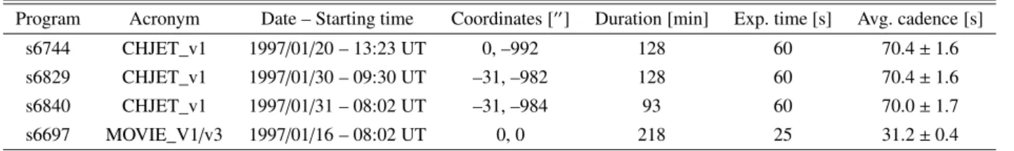
Table 1.Details of the CDS wide slit (90×240) observational programs, including their identification number, acronym, date and time of observation, center coordinates of the slit for that time in arcseconds, total duration in minutes, exposure time in seconds for each of the images and average time cadence in seconds with its standard deviation.
Program Acronym Date – Starting time Coordinates [] Duration [min] Exp. time [s] Avg. cadence [s]
s6744 CHJET_v1 1997/01/20 – 13:23 UT 0, –992 128 60 70.4±1.6
s6829 CHJET_v1 1997/01/30 – 09:30 UT –31, –982 128 60 70.4±1.6
s6840 CHJET_v1 1997/01/31 – 08:02 UT –31, –984 93 60 70.0±1.7
s6697 MOVIE_V1/v3 1997/01/16 – 08:02 UT 0, 0 218 25 31.2±0.4
of a specific solar region at a cadence of 1 image every 30 s, as seen by different spectral lines with different formation temper-atures. As images produced by close lines would overlap, we are constrained to the study of isolated and unblended lines. This mode has proven to be very useful in the study of dif-ferent solar features: blinkers, coronal jets, prominences, quiet Sun network and sunspots. The present BP observations were done in 1997 (see Table 1), using the wide slit in a sit-and-stare mode, i.e. the pointing is kept fixed and the plasma moves un-der the slit. Three bright lines of the NIS spectral range were used: He 584.34 Å, O 629.73 Å and Mg 368.07 Å. Their formation temperature in ionization equilibrium is re-spectively, in logarithmic scale, 4.5, 5.4 and 6.0 (Mazzotta et al. 1998; Young et al. 2003). The Mg line is blended with a Mg367.67 Å line which has a formation temperature of 5.9, therefore the image of the slit centered at 368 Å is the product of the BP emission in these two temperatures. Table 1 shows the details of these observations. Each NIS pixel corresponds to 1.68square, although the spatial resolution of CDS is closer to 6 (Pauluhn et al. 1999). A standard reduction was applied to the images in order to correct for bias, flat-field, cosmic rays and instrumental effects.
The BPs were visually identified in the Mg/window as compact regions with an enhanced emission over the sur-rounding corona. However, we note that network elements and blinkers can both have a coronal response (Gallagher et al. 1998). Leaving aside, for the moment, the possible link that could exist between both phenomena, we confirmed the BP na-ture by inspecting images from the Extreme ultraviolet Imaging Telescope (EIT). In these images, BPs are seen as point-like or loop-like structures that last for several hours (Zhang et al. 2001). All of them last for the whole CDS sequence, which varied between 93 and 218 min.
2.2. EIT
Images from the Extreme ultraviolet Imaging Telescope (EIT) were used to identify and follow the life evolution of the BPs. The BP corresponding to the CDS dataset s6744 can be iden-tified at≈13:00 UT on 20 January 1997 in the 171, 195 and 284 Å bandpasses, and remains still visible at 15:09 in the 195 Å band. For the s6829 dataset, the BP was a fuzzy en-hanced region at 7:00 UT in the 195 Å band that slowly be-came brighter and more recognizable by 9:00 UT. Its intensity was still increasing at 13:04 UT. For the s6840 dataset, the BP appeared some time between 5:00 UT and 7:00 UT (visible in
171, 195 and 284 Å bands). By 9:00 UT it had reached its max-imum brightness in 195 Å and was still visible at 13:00 UT, al-though fainter. The BP in dataset s6697 was visible for several hours (at least from 8 UT to 14 UT).
2.3. MDI
MDI (Michelson Doppler Imager) high resolution magne-tograms (0.6/pixel) were also analyzed for the BP observed on January 16 1997. They cover the whole CDS observational period with a cadence of one exposure per minute. The magne-tograms were corrected for differential solar rotation and for the geometrical projection of the line-of-sight magnetic flux (Chae et al. 2001; Hagenaar 2001). In order to increase the signal to noise, every five consecutive exposures were averaged result-ing in a final cadence of∼5 min.
3. Wavelet analysis
Fig. 1. Wavelet analysis results for the He 584 Å time series of the BP observed on January 20, 1997.Top panel: time variation of the number of counts after detrending; a sine function with a period of 822 s, corresponding to the peak in the wavelet analysis, is over-plotted.Middle panels: wavelet power spectrum with the cone of in-fluence over-plotted (cross-hatched region) and global wavelet. The dashed line represents the maximum period outside the cone of in-fluence. The periods corresponding to the first two maximums in the global wavelet are indicated below the graph, together with the as-sociated level of probability in brackets.Bottom panel: variation in time of the probability associated with the two strongest peaks in each time slice. The solid line is associated to the first maximum location (white dots on the power spectrum) and the dotted line to the second maximum (black dots). The 95% confidence level is given by the dot-dashed line.
moments of time. A randomization method is used to estimate the significance levels (O’Shea et al. 2001). The basic assump-tion of the method is that if there is no periodicity in the time-series, any order of the intensity values would be as likely as any other. By comparing the power spectrum obtained from the observed series to the one obtained from each of the permuta-tions in time of the intensity values, we can estimate the prob-ability p that a certain peak in the power spectrum would be produced by chance. We will consider as relevant signals those with a probability (1−p) greater than 95%. We calculated this probability for the global wavelet spectrum, an average in time of the power spectrum, and for the two strongest peaks (called first and second maximum) of each time slice. More details about the analysis can be found in Ugarte-Urra et al. (2004) or O’Shea et al. (2001).
We produced a light curve for each BP and each spec-tral window by integrating the emission coming from an area
of 3×3 or 4×4 pixels, depending on the exposure time, which increases the signal to noise without loss of spatial informa-tion due to the broad point spread funcinforma-tion of the instrument (Pauluhn et al. 1999). While for the case of the BP lo-cated at equatorial latitudes the region of integration was cor-rected for solar rotation, this correction was not necessary for the BPs located at the poles. The general trend of inten-sity increase/decrease of the light curves were subtracted from each BP with an appropriate running average in order to ana-lyze the variations that it experiences with respect to the trend. We describe now the results obtained for each of the BPs. The sequences with a 60 s cadence designed for coronal hole studies showed a saturation of the O629 Å BP counterpart, so the study could only be carried out on He 584 Å and Mg/368 Å. Special attention is given to the sequence of 30 s exposure where O 629 Å can be safely analyzed and where a comparison with high resolution MDI magnetograms is available.
3.1. January 20 dataset
This is one of the sequences run at polar coordinates. The BP appears in the He 584 Å window as a bright network ele-ment not very different from the surrounding area. Its emis-sion ranges between values comparable to those of other net-work elements and values 35% higher. In the Mg/window, the BP is clearly identified as a 20round structure with an in-tensity between 1.5−2 times the emission of the surrounding corona. The flux lightcurve was obtained from integrating the emission of the BP central part (3×3 pixels). The wavelet anal-ysis of the time-series shows an oscillatory pattern with a pe-riod of≈822 s at the beginning of the time-series in He584 Å. It extends over 3−4 complete cycles as can be seen in the sinusoidal dashed line plotted over the detrended time-series (Fig. 1, top panel). It is preceded and followed by two brighten-ings of a longer temporal response, of around 1000 s. The am-plitude of the intensity variations is of the order of 5−20%. The wavelet analysis shows that no oscillations are present above the probability threshold in the Mg/time-series. The am-plitude of the intensity variations (2−6%) are much smaller than those in He.
3.2. January 30 dataset
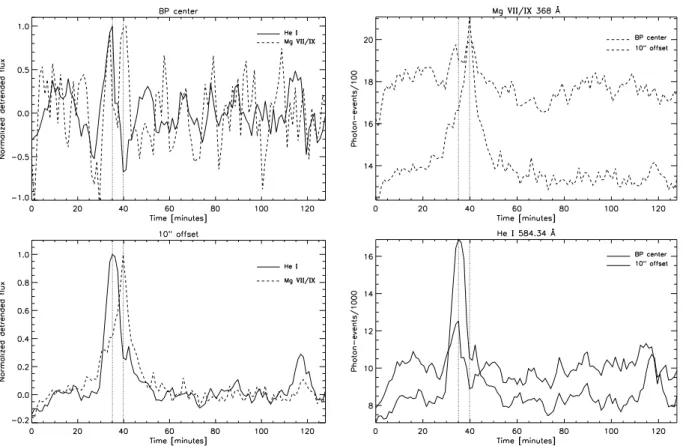
Fig. 2.He(solid line) and Mg/(dashed line) light curves of the BP observed on January 30. Two different locations are considered: BP center and an offset of 10 north of the BP center.Left panels: comparison of the temporal behaviour of the two spectral lines at the indicated location; the flux has been normalized to the maximum value of each curve to make the comparison easier.Right panels: comparison of the two locations for the same spectral line. The vertical dotted lines indicate the time when the events peaked in the off-center box.
We find intensity changes with amplitudes of the order of 4−10%, slightly lower than the previous dataset, and between 3−6% for Mg/.
The wavelet analysis reveals the presence of a band in the power spectrum corresponding to a period of 634−754 s for as long as 3 cycles. The probability ranges between 80 and 96%, perhaps indicative of a real oscillatory behavior, although it is below our initial probability requirements. Mg/does not show an oscillatory pattern in the power spectrum. It experi-ences, however, changes in the flux similar to the ones shown by He. The top left panel of Fig. 2 shows the detrended light curve for He(solid line) and Mg/(dashed line) normal-ized to their maximum values in order to make the comparison easier. Apart from the general trend, removed here, the figure shows common brightenings suggesting a connection between events at both temperatures.
There are, as well, events which are restricted to only one of the observed spectral lines, like the one which takes place in Mg/ 40 min after the start. This is an interesting event as seen in the wide slit movie. It is originated in a nearby network element that brightens and establishes an emission link, probably loops, with the element below the coronal BP. Unfortunately, the available resolution does not allow us to es-tablish this more firmly. The bottom left panel of Fig. 2 shows the light curve obtained from a box of integration located over the bridge between the network elements, north of the BP cen-ter. In He, this box is located 5 eastwards, as the peaks of
emission in He and Mg / are slightly offset. The right panels of Fig. 2 show the similar information, but this time we show in each graph the light curves of the two locations for the same spectral line. The vertical dotted lines indicate the time when the events peaked in the off-center box. The large rise in the Heflux (34% from trough to crest) starting at around 27 min after the beginning of the observations in the neigh-bouring network becomes visible in Mg/over the diffuse outskirts of the BP, 10−13 off-center, for just the duration of the event. The right panels show how the brightening, origi-nated off-center in He, produces a general rising of the coronal emission in the BP (center and offset), followed by a steeper increase, reaching 50%, at the top of that bridge and peaking 281 s after the initial He brightening. There is no such re-sponse in the Heemission after the first event. It soon regains its original flux, except for a little spike 143 s after the coro-nal peak. The ficoro-nal spike in the decay of the Heflux could be a response to the coronal emission. The formation of Heis still under discussion and one of the possible mechanisms is a reprocessing of EUV coronal radiation (Andretta et al. 2003).
3.3. January 31 dataset
Fig. 3.He584 Å and Mg/368 Å flux changes observed in a BP on January 31, 1997.Top two panels: flux variations for each of the lines.Bottom panel: both light curves have been detrended and normalized to its maximum value (He, solid line; Mg/, dashed).
elements which are 1.8−2.7 times brighter than the elements with no coronal counterpart.
The length of the time-series is only 93 min, shorter than previous datasets. The box of integration (3×3 pixels) was lo-cated in the center of the emission. The light curves obtained for both spectral lines are shown in the top two panels of Fig. 3, with the corresponding error bars obtained from the quadratic sum of the errors of individual pixels. The errors in individ-ual pixels were obtained from the standard formulae for NIS (Thompson 2000). The bottom panel shows a comparison of the variations experienced by the BP in both lines after de-trending and normalizing. These variations are very similar in both lines suggesting a connection between the events. Some of these events peak at the same time in both lines, but in other cases, like the one which peaks in Mg/25 min after the start or the one peaking at minute 48, are seen in Hewith some time delay. The delay is three datapoints (204 s) in the first case and two (143 s) in the second. Brightenings with no clear counterpart in the other line are present as well. The vari-ety of events suggests that the evolution of the flux in the BP (at this resolution) has a complex picture with different processes producing different observational patterns. The amplitudes of the variations are of the order of 5−18% for Heand 3−10% for Mg/.
The wavelet analysis results of the two time-series are shown in Fig. 4. The power spectrum (central panel) of both time-series has a high power band at around 700 s. In He, the peak is at a period of 688 s, while in Mg/it is at 750 s, with
a 99−100% confidence if we attend to the result of the wavelet analysis of the global wavelet spectrum. The time dependent plot of the probability shows, however, that certain parts of that band are below the 95% confidence level. In Hethe proba-bility is over 95% from minute 41 in the time-series. In the case of the coronal line, some points lie below the threshold, although most of the time around 95% confidence. The time-series can be reconstructed using its wavelet power spectrum, following the indications given by Torrence & Compo (1998). In this reconstruction, which basically sums the contributions of the different periods at the different times, we can disregard the higher periods thus revealing signals with lower periods. If we filter the periods greater than 1000 s, the confidence level rises above the threshold. Sinusoidal functions of periods 688 s and 719 s have been plotted over the detrended light curves (top panels of Fig. 4), where 719 s is the middle value between the 688 and 750 values that dominate the Mg/power spec-trum band. It stands out in the comparison that there is a reg-ularity in the appearance of the larger brightenings suggesting that a periodic phenomenon is taking place.
3.4. January 16 dataset
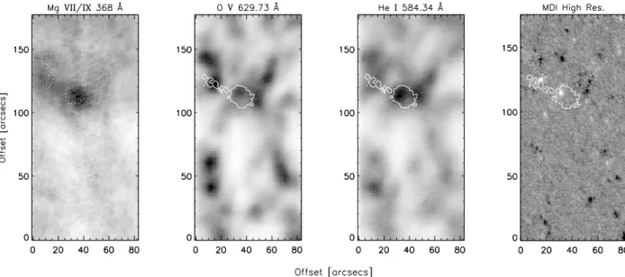
This bright point, located at Sun center, is visible for several hours in EIT (at least from 8 UT to 14 UT) and it appears as a point structure of 3×3 pixels in the 195 Å passband. Figure 5 shows the appearance of the BP in the CDS wide slit images. In Mg/368 Å, we see it as a diffuse elliptical cloud with enhanced emission 2.1−2.5 times over the background. In O629 Å we can identify between 2 and 4 network elements (depending on the instance) at the junction of three network cells. The network elements present high variable emission and their increase/decrease is not always simultaneous. He584 Å images are very similar to the Oimages with the network el-ements clearly delimiting the edges of the cells. A MDI high resolution magnetogram is also displayed in the figure and the contours of the Mg /and He emission are over-plotted for comparison. A bipolar region associated with the coronal emission and dominated by the negative fragments is present. As we see in the O and He ı images, there are other bright network elements in the field of view, but they do not have a coronal counterpart in Mg/. It is easy to notice that the coronal emission is associated with the presence of strong op-posite polarities. The positive fragments associated with the BP and the surrounding bright area have peaks in the magnetic flux density between 97 and 187 Mx cm−2, while the positive frag-ment seen at an offset of (15, 65) (associated with the bright Onetwork element) does not reach 40 Mx cm−2.
Fig. 4.Wavelet analysis results of the BP observed on January 31, 1997 at 08:02 UT. The left panel corresponds to the He584.34 Å time-series and the right panel to Mg/368 Å. The dashed lines plotted over the two light curves at the top panels account for sinusoidal functions with periods of 688 and 719 s respectively, corresponding to the peaks of the power spectrum.
Fig. 5.CDS wide slit images in Mg/368 Å, O629.73 Å and He584.34 Å, of the coronal bright point observed on January 16, 1997, plus a MDI high resolution magnetogram. In the images, black regions are the brightest sources and white the faintest. In the magnetogram, positive polarities are in white and negative in black. All images were taken at 10:01 UT. Solid (Mg/) and dotted (He) contours are used as a reference for comparison.
general BP emission increases monotonically all along the ob-servation period and that the variability is higher as the emis-sion increases. This general trend has been removed, using an appropriate running average for each of the light curves, in or-der to study the variations with respect to the trend. The ampli-tude of these variations are of the order of 3−11% in the case
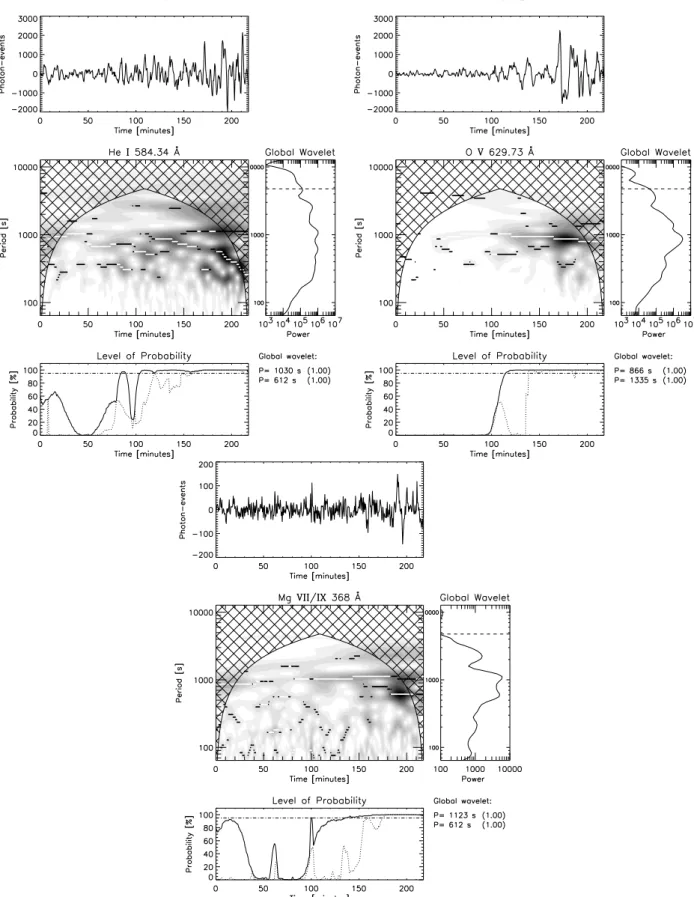
Fig. 6.Wavelet analysis results of the BP observed on January 16, 1997 at 08:02 UT. Top left panel corresponds to the He584.34 Å time-series, top right to the O629.73 Å ones and bottom to the Mg/368 Å blend.
the time series, but it does not last for more than two cycles in any of the periods. There is, however, a peak in the power spectrum at around 1123 s that lasts for 63 min, with the first two cycles well outside the cone of influence. Simultaneous to
Fig. 7.Section of a five minute averaged MDI high resolution magnetogram showing the photospheric magnetic configuration associated to the Mg/BP observed on January 16, 1997. On the left panel, the solid and dotted contours locate the Mg/and Oemission, respectively. The section is a close-up of the region centered at approx. (45, 120) in Fig. 5. White accounts for positive magnetic flux density,φ, and black for negative. In the center and right panels we plot only those pixels with|φ| ≥21 Mx cm−2. The right panel shows the maximum change in
orientation (∼20◦) of the straight line joining the centroid positions of the two opposite polarities for two different images. White/black contours correspond in this case to the negative/positive polarity.
analysis to the un-detrended light curve and reconstructed it us-ing the power spectrum with only the shorter periods taken into consideration. We find similar results, which give us confidence that the peaks in the power spectrum have a solar origin.
The analysis of the Olight curve shows a power spectrum with certain similarities to He. A band with a confidence level over the 95%, with periods ranging between 944 and 794 s, ap-pears at the same time as the diagonal band in He, suggesting a connection between the events. In this case, the peak in the power spectrum at 944 s can host around 3 oscillatory cycles. The same occurs for the peak at 364 s simultaneous to the one found for Heat 306 s.
In the case of Mg/we can clearly identify, at the bot-tom panel of Fig. 6, the band peaking at 1123 s that we found in the Hedata. It is long enough to host 4 complete cycles, 3 of them outside the cone of influence. The shorter periods, 216 s, barely seen in the figure can also be detected in this case using the reconstruction technique, but only marginally and for less than two cycles over the 95% confidence level. Somehow, the fact that they are present at the same location as in the cooler lines suggests that they could be real and therefore could be part of the coronal evolution of the BP. The lower signal to noise of this spectral line and the mixture of different structures with the current spatial resolution are all possible causes that this oscillation is partially hidden in Mg/. Finally there is an-other period peaking at 612 s, close to the end of the temporal sequence.
4. Magnetic field evolution
It was noted in the introductory section the importance of the evolution of the magnetic fragments and the associated magnetic flux in relation to the BP appearance (see also Ugarte-Urra et al. 2004). We feel that the present discussion will benefit if we discuss the EUV brightness fluctuations in the context of the changes experienced by the magnetic field.
We do it, therefore, for one of the BPs for which we have MDI high resolution magnetograms.
The MDI high resolution magnetograms (0.6/pixel) are available for the BP observed on January 16. The observations cover the whole CDS observing time with a cadence of one magnetogram every minute. In order to improve the signal to noise we produced new magnetograms by averaging five con-secutive images, which left us a final cadence of five minutes. The noise in the dataset can be obtained from the core of the distribution function of flux densities,φ(Hagenaar 2001). This core is well described by a Gaussian fit, which reveals in our case a level of noise ofσ=11.1 Mx cm−2.
The magnetic configuration of the BP area is visible in Fig. 5 (right panel). The left image in Fig. 7 shows a close-up of the region centered approximately at the offset coordinates of (45, 120) in Fig. 5, with the Mg/and Oisocontours to make the comparison easier. The alignment between CDS and MDI was done using the header coordinates. The uncertainty is not larger than 5. There is a main negative polarity made of several fragments that dominates and three satellite positive po-larities around it, one of them stronger than the others, see A in Fig. 7. The corresponding Oand Heimages show three net-work elements associated with the three points where opposite polarities are confronted. Attending to the evolution of these satellite polarities we find in the images from 2 to 4 network elements associated with the coronal emission, which mainly lies over the left interaction point, A. The movie, made with the collection of images, shows an approaching movement of the two polarities, A and B, at this location, as well as a disap-pearance or cancellation of the lower positive fragment.
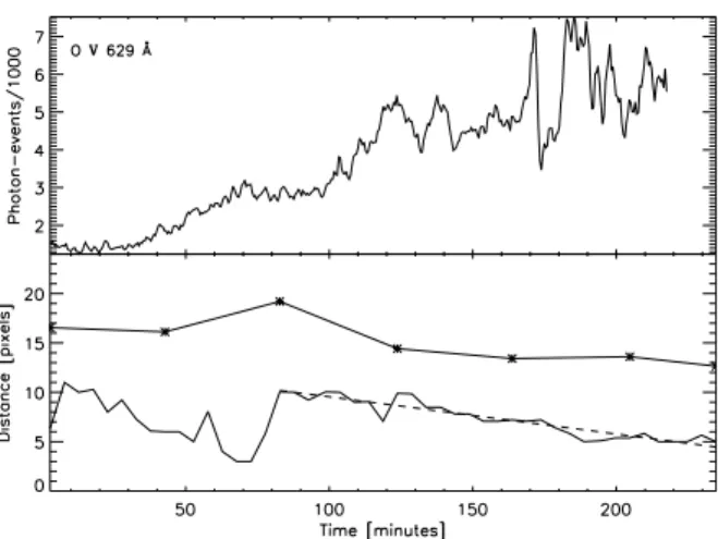
Fig. 8.Comparison between the temporal variation in the transition region emission of O629.73 Å (top) and the distance between oppo-site polarities A and B (bottom). The asterisks account for the distance between centroids and the single solid line represents the distance be-tween the closest pixels. The dashed line is a linear fit to the second distance decrease section used to determine the approaching velocity of 0.27 km s−1.
probability for a certain variate to be greater than a certain value. In this case the variate is the magnetic flux density. From the ratio of the two survival functions we obtained the propor-tion of pixels associated with noise for the different flux density values. At 21 Mx cm−2less than 1% of the pixels are associated
with noise. We adopt this as our working value. We plot in the center and right panels of Fig. 7 the BP magnetic configuration considering only those pixels with|φ| ≥21 Mx cm−2.
We determined then the distance between A and B all along the time-series in two ways. First of all, we calculated the dis-tance between the two closest pixels with a magnetic flux that we know for certain it is not associated with noise, i.e. those pixels with |φ| ≥ 21 Mx cm−2. Secondly, we calculated the
distance between the centroids of both polarities at different instances of the time-series. Both results are shown in Fig. 8, together with the temporal changes in the number of counts (photon-events) in the transition region line. Asterisks repre-sent centroid distances, while the single solid line accounts for the distance between closest pixels. The approaching trend is clear in both curves. The latter shows two different sections of decreasing distance joined by a steep increase at around 80 min after the start of the observing period. This increase is due to the cancellation of the positive fragments that we see detached from the main positive polarity in the left and center panels of Fig. 7. After the disappearance of these fragments, the clos-est pixel belongs to the largclos-est positive fragment in the figure, which is further apart. The separation between centroids shows a similar profile due to the same phenomenon. This is the dis-tance between the strongest flux concentrations since we only consider pixels with a flux over 21 Mx cm−2. The real distance
between opposite polarity fragments would probably be less than that. A comparison with the CDS emission reveals that the approach of the polarities is followed by an increase in the transition region flux. Interestingly, the flux increase reaches a 30 min “plateau” when the distance between polarities expe-riences the steep increase, and as soon as it starts to decrease
Fig. 9.Comparison between the EUV variability of the BP detrended emission, as obtained from the CDS wide slit images, and the mag-netic flux of the two opposite polarities. Shaded areas point out loca-tions where we see a decrease in the positive flux preceding a bright-ening in the EUV lines. The local minimum is given by a dashed line.
again, the flux rises. Another characteristic is that the amplitude of the Obrightenings becomes larger with time. The fact that the closest distance between polarities is reached just before the “plateau” phase and the amplitudes are not the largest at this moment, suggests that the proximity of the centroid, or in other terms the bulk of the positive magnetic flux, is more important in terms of energy release. From these plots we can infer the approach velocity. From a linear fit (Fig. 8) to the second sec-tion of the curve that gives the distance between closest pixels (i.e. when the small fragments have already been canceled), we find a velocity of approach of 0.27±0.02 km s−1. In the case
of the centroids, we obtain a value of 0.15±0.06 km s−1using
all the points. If we just fit the points after the small fragments have canceled the result is 0.26±0.09 km s−1. These results are inside the range of typical values (0.1−0.3 km s−1) quoted by Priest et al. (1994).
and B. From this comparison the first thing that we notice is that the monotonic increase of the EUV emission, visible in Fig. 8 for Oand similar for the other two lines, is associated in Fig. 9 with a decrease in the positive magnetic flux, which is an order of magnitude larger than the negative one. On smaller timescales, the plot suggests that sudden decreases in the posi-tive magnetic flux (shaded areas) seem to take place just before (or during the rising phase) a brightening is observed in the transition region or the corona, and sometimes both. The lo-cation of the local minimum in the magnetic flux is given by a dashed line. These results could suggest that magnetic flux can-cellation are associated to the stronger brightenings and give support to the picture that proposes reconnection as the main process producing the appearance of BPs and its characteris-tic variability (Priest et al. 1994; Longcope 1998). However, we feel that more observations are needed to confirm a definite correspondence between decreases in the magnetic flux of this order and the brightenings. The negative flux does not show as good correlation as the positive one, but this could be explained by the fact that fragment B is weaker in flux and also belongs to a more complex structure, where the surrounding positive frag-ments (see Fig. 7) could play an active role in the evolution.
5. Discussion
It is clear from the present work and that of Madjarska et al. (2003) and Ugarte-Urra et al. (2004) that BPs have intermittent (few cycles), but clearly defined periods of oscillation ranging from around 400 s up to 1100 s (0.9−2.5 mHz) in upper chro-mospheric, transition region and sometimes coronal plasma. In the case of one BP, periods as short as 236 s (4.2 mHz) were also detected. Apart from the clear oscillatory cases, we have found several other cases with similar periods where the prob-ability estimates do not reach the required 95%, but they are very close. We believe that some of these oscillations are real, in particular those detected simultaneously in several spectral lines, but are hidden in the low spatial resolution of the inte-grated emission.
Oscillations in the quiet Sun chromosphere have been known for a long time and is a well documented phenomenon. Two regions showing two different characteristic frequency ranges are normally differentiated. On one side the∼5.5 mHz (3 min) oscillations seen in the chromospheric internetwork (Dame et al. 1984; Carlsson et al. 1997; Curdt & Heinzel 1998; Krijger et al. 2001; Wilhelm & Kalkofen 2003, and ref-erences therein); on the other, the network lanes and the net-work bright points (NBPs), which show a wider range of fre-quencies (0.8−3.3 mHz), 5−20 min periods according to Lites et al. (1993; but see also Dame et al. 1984; Curdt & Heinzel 1998; Doyle et al. 1999; Banerjee et al. 2001; McAteer et al. 2002, 2003). The four BPs analyzed here lie on the network lanes and their O and He counterparts are network ele-ments generally indistinguishable from other eleele-ments with no coronal counterpart. The first thing that we notice is that the frequencies found for these BPs lie in the frequency range of the chromospheric network oscillations. One characteristic of NBPs is that they are associated with photospheric mag-netic flux elements (Cauzzi et al. 2000). This can be clearly
seen in Fig. 2 of McAteer et al. (2003), which shows the ap-pearance of several NBPs at different temperatures in the solar atmosphere, from the chromosphere, through the transition re-gion to the corona, co-aligned with a magnetogram. It is worth noting that McAteer et al. (2003) NBP 5 shows the charac-teristic size and enhanced coronal emission overlying two op-posite polarity magnetic fragments of a coronal bright point (with a peak emission around 2 times higher than the surround-ing corona, as checked from the original image). In the tran-sition region image we see two bright features at the location where the footpoints of the coronal loop would be, connected by what looks like a cooler loop structure; these footpoints can be traced into the chromosphere and the two opposite polarities in the magnetogram. Only the brightest one was the subject of the NBP study by the authors. Figure 2 in Cauzzi et al. (2000) shows a similar configuration with two opposite magnetic frag-ments of reasonable strength for a coronal bright point, sepa-rated by less than 10, below the chromospheric emission of two NBPs. No coronal image is available in this case. More images can be compared in Nindos & Zirin (1998).
This leads us to the conclusion that a fraction of the NBPs (and the associated magnetic field) are most likely the foot-points of the tiny loops which comprise coronal bright foot-points (Sheeley & Golub 1979); the cool footpoints of loops which rise to greater temperatures (Cook et al. 1983). This would explain why we see the same periodicities in both features. Recently, McAteer et al. (2004), analyzing quiet Sun network and internetwork TRACE oscillations, found that the network has a peak occurrence rate periodicity of 231−346 s, with a sig-nificant tail of higher period oscillations (as long as∼1000 s). The peak decreases in occurrence rate in the highest formation temperature passband (≤1×10⁵K) suggesting that the waves may dissipate, shock, move away from the network or change frequency. Gouttebroze et al. (1999) did not find signature of 2.5−7 mHz (period of 143−400 s) oscillations in lines with a temperature formation≥5×10⁴K. If we bear in mind that BP’s
studies (Ugarte-Urra et al. 2004,and the present one) show os-cillations with typical periods of around 400−1100 s, with only one case showing shorter periods, all this seems to be consis-tent with a picture where only the longer periods observed in the chromospheric NBP, assumed here as the footpoints of hot-ter loops, make it through to the transition region and corona. However, more observations with simultaneous chromospheric and coronal counterparts of the BP will be needed to confirm that.
Different interpretations are given for these long frequency oscillations in the chromospheric network, which show no sign of distinctive peaks in the power spectrum (Krijger et al. 2001); namely, in terms of formation of standing waves by inter-nal gravity waves (Deubner & Fleck 1990; Lou 1995) or up-ward propagating MHD waves excited by granular motions (Kalkofen 1997; Hasan & Kalkofen 1999), although more dis-cussion is still needed (Musielak & Ulmschneider 2003).
Although we should note that the formation of He line is still under discussion (Andretta et al. 2003). We see periods of around 600 s in Oand Heoverlapping. The January 16 BP is the clearest case with certain periods shared by two of the three lines in the sample (He, O and Mg/). How are these oscillations related to the heating of BPs and how do they merge with the idea that reconnection plays a dominant role in the evolution of BPs?
One idea is that the observed intensity oscillations are asso-ciated with compressible waves, e.g. the acoustic mode which has been identified in coronal structures as both a propagating wave (e.g. Nakariakov et al. 2000) and standing waves (e.g. Ofman & Wang 2002) or the fast mode. An alternative interpre-tation, as a kink mode observed through the modulation of the observed width of the structure guiding the wave (Cooper et al. 2003), may be excluded from consideration as it is not likely that the kink mode, practically incompressible, has a notice-able amplitude in the chromosphere and the transition region.
The mode oscillates between the footpoints of the magnetic field line. Along the field line, the sound speed changes, but for the global mode (or any other lower harmonics) it is the aver-age sound speed which determines the period, not the local one, hence this would mean that the oscillations have a collective na-ture, e.g., similar to the global acoustic mode of a coronal loop (Ofman & Wang 2002) or their second harmonics (Nakariakov et al. 2004). The common feature of these oscillations is the positioning of nodes of the velocity perturbations and maxima of density perturbations at the lower layers of the atmosphere. In particular, in the structure of the global acoustic mode is
Vz(s,t)∝cos
πC s L t cos π Ls , (1)
ρ(s,t)∝sin
πC s L t sin π Ls , (2)
whereCsis a speed of sound,Lthe loop length, andsis a
dis-tance along the loop with the zero at the loop top. According to Eqs. (1) and (2), the oscillation period is given by the expres-sion 2L/Cs. As the magnetic field in a coronal bright point is
closed, it may be considered as a small loop with the oscillation modes described by these equations. On the other-hand, if the magnetic topology of the bright point is more complicated than the loop geometry, its “building elements” may be modelled as individual loops. In addition, as the acoustic wave considered here propagated strictly along the magnetic field, it does not feel the magnetic field complexity, simply following the local line.
Suppose the length of the loop forming an oscillating bright point is 30 Mm (corresponding to a 10 Mm radius), the global acoustic mode with periods of about 600 s would require the sound speed to be 100 km s−1. This value of the sound speed
is certainly reasonable. The period of the second harmonics of this loop is 300 s, also in the observed range. Different periods can be easily explained by different loop lengths and by slightly different profiles of the sound speed along the loop (grow-ing from the chromospheric 30 km s−1to coronal 150 km s−1).
Also, a lower lying loop would in general have lower sound speed.
The domination of the oscillations in chromospheric and TR emission lines, is consistent with this interpretation too: ac-cording to Eq. (2) the density perturbations are stronger near the loop footpoints. At the coronal heights, the oscillations are not so pronounced because the density oscillations have a node at the loop apex.
Another possible interpretation of these oscillations is that they are connected with vertically propagating fast magneto-acoustic waves trapped between the dense chromosphere and the upper boundary of the bright point magnetic structure, where the Alfvén speed experiences a sharp increase. The wavelength of such waves is about double the radius of the closed magnetic field lines, and the characteristic speed is sev-eral sound speeds (the lowest possible value is one and a half sound speed, in the case of β = 1). Taking the values from the previous example, we obtain the longest characteristic pe-riod of about 130 s (for the radius 10 Mm and the sound speed 100 km s−1). This value is less consistent with the observational
findings than the periods given by the acoustic model.
This simple model then suggests that the bright point os-cillations could be associated with the global acoustic modes of closed magnetic structures associated with the bright point. However, this does not address the important question of how these waves are generated. They could be related to the super-granular motions or may be excited by the energy deposition from the reconnection process. This second scenario would be supported by the fact that, in the case of the BP observed on January 16, we detect sudden decreases in the magnetic flux at the same time as the oscillations in the EUV flux take place.
If reconnection is important in BPs (as commonly assumed) it has to be a slow process as the observed Doppler shift of tran-sition region lines is at most 10 km s−1red-shifted (Madjarska et al. 2003; Xia et al. 2003; Popescu et al. 2004) compared to a red-shift of 10−25 km s−1 for blinkers (Madjarska & Doyle
2003) and±100 to 200 km s−1(Madjarska & Doyle 2002) for
bi-directional jets. It is more in the order of the quiet Sun net-work (Teriaca et al. 1999) which has a red-shift of 8−10 km s−1
at these temperatures.
In this respect we may have a problem. As shown in Sect. 4, the converging speed of the two polarities was measured as 0.27 km s−1 which is an excellent agreement with a study by
Chae et al. (2002a) who measured the approach for two dif-ferent observations of converging polarities. In one instance the speed was 0.35 km s−1, while the other was 0.27 km s−1. In follow-up work, Chae et al. (2002b) considered two nection models, the Sweet-Parker model and the faster recon-nection Petschek model. They showed that the Sweet-Parker model does not have inflow speeds greater than 0.08 km s−1
while in the Petschek model, the inflow speed equals the ob-served speed just below the temperature minimum. Higher up in the atmosphere, e.g. the chromosphere and transition region, the speeds are in the range 20 to 100 km s−1. Thus, although the
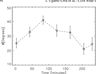
Fig. 10.Variation in time of the angle between the line joining the centroids of the two polarities of the January 16 BP andS olar_Y=0.
in the model. For example, taking a very small magnetic fill-ing factor (∼0.05) and a small electric conductivity of 1010s−1
yields an inflow speed of 0.27 km s−1which would be
consis-tent with the observations (Chae et al. 2002a,b). However, even the Sweet-Parker model gives large velocities in the upper at-mosphere. Thus this would rule out both of these as possible reconnection models for BPs.
Binary reconnection, an interaction of pairs of unbalanced sources has been proposed (Priest et al. 2003) as a fundamen-tal mechanism to produce coronal heating. One aspect of this mechanism is that the relative motions of the sources are likely to build-up twisted force-free structures that relax by turbulent reconnection resulting in heating. We have tested this possible scenario against the BP observed on January 16. The sources show a relative motion of approach, as described earlier, but also of rotation (right panel of Fig. 7). We have measured the angle that the line joining the two centroids makes with the
Solar_Y = 0 (Fig. 10). The figure shows how one source ro-tates with respect to the other reaching a maximum of 41◦ and then returning to the original configuration. The error bars come from the uncertainty in the determination of the centroid, assumed as 1 pixel. The energy injected by this rotation can be determined using ∆E = F2∆θ2/(24π2µL
eff) (Priest et al.
2003) withFthe magnetic flux of the weakest polarity,∆θthe angle change,µthe magnetic permeability andLeff the eff
ec-tive length of the magnetic field lines. The maximum change in orientation is∆θ∼20◦and takes 122 min. ChoosingLeffas
10.2 Mm (15 MDI pixels for the footpoint separation and semi-circular loop shape) and a range of magnetic flux values rang-ing from 7.8×10¹⁷to 7.2×10¹⁸Mx (that depend on the
thresh-old of integration) for the weakest polarity, we obtain an energy injection per second of≈1018−1020erg s−1, much smaller than
the typical values (1023−1024 erg s−1) of energy loss in BPs
(Habbal & Withbroe 1981; Priest et al. 1994; Longcope et al. 2001). A magnetic flux of 1.4×10²⁰ Mx would be required
under these conditions, an order of magnitude larger than the positive polarity flux. The uncertainty in the different values can not explain the disagreement, therefore we conclude that the heating of this BP can not be explained by a helicity injec-tion process.
6. Conclusions
We have studied CDS wide slit movies of four coronal bright points (BPs) in three spectral lines: He 584.34 Å, O 629.73 Å and Mg/ 368 Å. The BPs can be clearly identified in the Mg/images where they have a peak emis-sion between 1.8−2.7 the flux of the surrounding corona. This identification is not straightforward for the cooler lines, where the emission and appearance can be similar to that of other net-work elements. The BPs show flux fluctuations with an ampli-tude generally ranging 4−20% in He584.34 Å, 10−20% in O 629.73 Å and 2−10% in Mg/368 Å, although there are brighter events where the percentage could reach the 50% increase.
The wavelet analysis of the time-series confirms the oscil-lating nature of the BP’s emission in EUV lines (Ugarte-Urra et al. 2004). We find wavetrains with periods ranging between 600−1100 s in all three lines. We find as well, in one of the BPs, periods as short as 236 s. We notice that these periods lie in the period range of the chromospheric oscillations and we conclude that a fraction of the network bright points that are observed in the chromospheric network are most likely the cool footpoints of the loops that coronal BPs are made of.
In the case of one BP, for which MDI high resolution mag-netograms were available, we have found that the increase in the EUV flux and its variability takes place as the mag-netic polarities approach and the dominant (positive) flux de-creases. Sudden magnetic flux decreases are observed at the same time as the oscillations in the EUV emission become sig-nificant. This would support a scenario where the waves, in-terpreted here in terms of global acoustic modes, are driven by magnetic reconnection events. However, Sweet-Parker and Petschek models do not seem to explain the typical small Doppler shift values characteristic of BPs. We believe that a new model is needed in order to explain these Doppler shift values in the context of magnetic reconnection, where waves play also a very important role.
Acknowledgements. Research at Armagh Observatory is grant-aided by the N. Ireland Dept. of Culture, Arts and Leisure. This work was supported by PPARC grant PPA/V/S/1999/00668. CDS, EIT and MDI are instruments onboard SoHO which is a project of international co-operation between ESA and NASA. We would like to thank the ref-eree for useful comments and suggestions that helped us improve the presentation of the paper.
References
Andretta, V., Del Zanna, G., & Jordan, S. D. 2003, A&A, 400, 737 Aschwanden, M. J. 2003, in NATO Advanced Research Workshops:
Turbulence, Waves and Instabilities in the Solar Plasma, 215 Banerjee, D., O’Shea, E., Doyle, J. G., & Goossens, M. 2001, A&A,
371, 1137
Banerjee, D., O’Shea, E., Goossens, M., Doyle, J. G., & Poedts, S. 2002, A&A, 395, 263
Carlsson, M., Judge, P. G., & Wilhelm, K. 1997, ApJ, 486, L63 Cauzzi, G., Falchi, A., & Falciani, R. 2000, A&A, 357, 1093 Chae, J., Wang, H., Qiu, J., et al. 2001, ApJ, 560, 476
Chae, J., Moon, Y., Wang, H., & Yun, H. S. 2002b, Sol. Phys., 207, 73 Cook, J. W., Brueckner, G. E., & Bartoe, J.-D. F. 1983, ApJ, 270, L89 Cooper, F. C., Nakariakov, V. M., & Williams, D. R. 2003, A&A, 409,
325
Curdt, W., & Heinzel, P. 1998, ApJ, 503, L95
Dame, L., Gouttebroze, P., & Malherbe, J.-M. 1984, A&A, 130, 331 Deforest, C. E., & Gurman, J. B. 1998, ApJ, 501, L217
De Moortel, I., & Hood, A. W. 2000, A&A, 363, 269 Deubner, F.-L., & Fleck, B. 1990, A&A, 228, 506
Doyle, J. G., van den Oord, G. H. J., O’Shea, E., & Banerjee, D. 1999, A&A, 347, 335
Egamberdiev, S. A. 1983, Soviet Astron. Lett., 9, 385
Gallagher, P. T., Phillips, K. J. H., Harra-Murnion, L. K., & Keenan, F. P. 1998, A&A, 335, 733
Gouttebroze, P., Vial, J.-C., Bocchialini, K., Lemaire, P., & Leibacher, J. W. 1999, Sol. Phys., 184, 253
Habbal, S. R., & Withbroe, G. L. 1981, Sol. Phys., 69, 77
Habbal, S. R., Withbroe, G. L., & Dowdy, J. F. 1990, ApJ, 352, 333 Hagenaar, H. J. 2001, ApJ, 555, 448
Harrison, R. A., Sawyer, E. C., Carter, M. K., et al. 1995, Sol. Phys., 162, 233
Hasan, S. S., & Kalkofen, W. 1999, ApJ, 519, 899 Kalkofen, W. 1997, ApJ, 486, L145
Krijger, J. M., Rutten, R. J., Lites, B. W., et al. 2001, A&A, 379, 1052 Lites, B. W., Rutten, R. J., & Kalkofen, W. 1993, ApJ, 414, 345 Longcope, D. W. 1998, ApJ, 507, 433
Longcope, D. W., Kankelborg, C. C., Nelson, J. L., & Pevtsov, A. A. 2001, ApJ, 553, 429
Lou, Y. 1995, MNRAS, 274, L1
Madjarska, M. S., & Doyle, J. G. 2002, A&A, 382, 319 Madjarska, M. S., & Doyle, J. G. 2003, A&A, 403, 731
Madjarska, M. S., Doyle, J. G., Teriaca, L., & Banerjee, D. 2003, A&A, 398, 775
Marsh, M. S., Walsh, R. W., & Bromage, B. J. I. 2002, A&A, 393, 649 Mazzotta, P., Mazzitelli, G., Colafrancesco, S., & Vittorio, N. 1998,
A&AS, 133, 403
McAteer, R. T. J., Gallagher, P. T., Williams, D. R., et al. 2002, ApJ, 567, L165
McAteer, R. T. J., Gallagher, P. T., Williams, D. R., et al. 2003, ApJ, 587, 806
McAteer, R. T. J., Gallagher, P. T., Bloomfield, D. S., et al. 2004, ApJ, 602, 436
Musielak, Z. E., & Ulmschneider, P. 2003, A&A, 406, 725
Nakariakov, V. M., Verwichte, E., Berghmans, D., & Robbrecht, E. 2000, A&A, 362, 1151
Nakariakov, V. M., Tsiklauri, D., Kelly, A., Arber, T. D., & Aschwanden, M. J. 2004, A&A, 414, L25
Nindos, A., & Zirin, H. 1998, Sol. Phys., 179, 253 Ofman, L., & Wang, T. 2002, ApJ, 580, L85
O’Shea, E., Banerjee, D., Doyle, J. G., Fleck, B., & Murtagh, F. 2001, A&A, 368, 1095
Parnell, C. E. 2002, MNRAS, 335, 389
Pauluhn, A., Rüedi, I., Solanki, S. K., et al. 1999, Appl. Opt., 38, 7035 Popescu, M. D., Doyle, J. G., & Xia, L. 2004, A&A, in press Priest, E. R., Parnell, C. E., & Martin, S. F. 1994, ApJ, 427, 459 Priest, E. R., Longcope, D. W., & Titov, V. S. 2003, ApJ, 598, 667 Sheeley, N. R., & Golub, L. 1979, Sol. Phys., 63, 119
Teriaca, L., Banerjee, D., & Doyle, J. G. 1999, A&A, 349, 636 Thompson, W. T. 2000, CDS Software Note N◦49
Torrence, C., & Compo, G. P. 1998, Bull. Amer. Meteor. Soc., 79, 61 Ugarte-Urra, I., Doyle, J. G., Madjarska, M. S., & O’Shea, E. 2004,
A&A, 418, 313
Wilhelm, K., & Kalkofen, W. 2003, A&A, 408, 1137 Xia, L. D., Marsch, E., & Curdt, W. 2003, A&A, 399, L5