Using Features Of Models To Improve
State Space Exploration
Author
A.R. HeijblomSupervisors
Prof. Dr. J.C. van de Pol Dr. Ir. M. van Keulen J.J.G. Meijer MSc
Master Thesis
Submitted December 14, 2016
Faculty of Electrical Engineering, Mathematics and Computer Science
Abstract
State space methods are a popular approach to perform formal verification. However, these methods suffer from the state space explosion problem. In the past decades many methods did arise to cope with the state spaces of larger models. As result, a user has many different strategies in which state space methods can be applied on new models.
Due to the wide variety of strategies and models is may be hard for a user to select an appropriate strategy. If a bad strategy is selected, the given model can be unsolvable or the process may waste resources like time and memory. Moreover, the intervention of the user makes state space methods less automated. Therefore, it would be convenient if model checking tools itself determine the strategy for a given model. In this way, model checking tools can determine the most suitable strategy for a given model such that the available resources are optimally utilized.
This process requires model checking tools to predict a strategy based on the information presented in a given model. Our research investigates to what extent characteristics of a model can be used to predict an appropriate strategy. The performance of 784 different PNML and DVE models was determined using
LTSminfor 60 selected strategies. This information was used to create several classifiers using machine learning techniques. The classifiers should predict an appropriate strategy given eleven selected features of a model.
Preface
The past year I’ve worked on a graduation project of the Master Computer Science at the University of Twente. The results of this project are discussed in this thesis. During the project, I learned a lot about the techniques I used, which were mostly new to me. I discovered how simple tools like bash could make tasks much easier than performing it manually. Due to the massive amount of data, programming and automating tasks were necessary and I definitely enjoyed writing the many programs and scripts needed to collect and analyze the data.
I would like to thank Jeroen for guiding me during the project. During the first weeks, he taught me many things about LTSmin and provided the necessary tools to start my project. He was always there for me in providing information I needed to advance my project.
I would also like to thank my supervisors for the guidance during my project. The meetings were valuable to me to shape my project and their feedback was very useful to improve and advance my project.
Last but not least, I would like to thank my family and friends. In the past months, they were always there for me. They helped to keep me motivated and supported me during the project.
Contents
Abstract 1
Preface 2
Contents 3
1 Introduction 6
1.1 Background . . . 6
1.1.1 Verification Methods . . . 6
1.1.2 State Space Methods In Practice . . . 7
1.2 Goals . . . 8
1.3 Approach . . . 8
1.4 Structure Of Thesis . . . 9
2 Preliminaries - LTSmin 10 2.1 Tool Overview . . . 10
2.2 Front-end Modules . . . 10
2.3 Wrapper Modules . . . 11
2.4 Back-end Modules . . . 11
2.5 Summary . . . 11
3 Preliminaries - Machine Learning 12 3.1 Overview . . . 12
3.1.1 Supervised Learning . . . 12
3.1.2 Unsupervised Learning . . . 13
3.1.3 Reinforcement Learning . . . 13
3.2 Classifier Creation . . . 13
3.3 Classification Algorithms . . . 14
3.3.1 Decision Trees . . . 14
3.3.2 K-Nearest Neighbors . . . 14
3.3.3 Support Vector Machines . . . 15
3.4 Binary Classifier Evaluation . . . 15
3.4.1 2×2 Confusion Matrix . . . 15
3.4.2 Metrics . . . 15
3.4.3 Example - Spam Filter . . . 17
3.5 Multiclass Classifier Evaluation . . . 18
3.5.1 n×nConfusion Matrix . . . 18
3.5.2 Transformation To 2×2 Confusion Matrix . . . 18
3.5.3 Metrics . . . 19
3.5.4 Example - Simple Handwriting Recognition . . . 20
3.6 Metrics For Cost-sensitive Classifiers . . . 21
3.6.1 Metrics . . . 21
4 Related Work 24
4.1 Symbolic State Space Methods . . . 24
4.2 Improvements Of State Space Methods . . . 24
4.2.1 BDD Construction . . . 25
4.2.2 Partitioning Of Transitions . . . 25
4.2.3 State Space Traversal Techniques . . . 25
4.2.4 Saturation . . . 26
4.3 Strategy Prediction . . . 26
5 Research Questions 27 5.1 Main Question . . . 27
5.2 Research Question 1 . . . 27
5.3 Research Question 2 . . . 28
5.4 Research Question 3 . . . 28
5.5 Summary . . . 28
6 Methods 29 6.1 Scope . . . 29
6.1.1 Selected Strategies . . . 29
6.1.2 Selected Features . . . 31
6.2 Techniques . . . 32
6.2.1 Model Collection . . . 32
6.2.2 Tools And Programs . . . 32
6.2.3 Machines . . . 33
6.3 Method . . . 33
6.3.1 Running State Space Exploration Tests . . . 33
6.3.2 Processing Data . . . 34
6.3.3 Analyzing Performance Data . . . 36
6.3.4 Creating And Evaluating Classifiers . . . 36
6.3.5 Feature Relevance Analysis . . . 37
7 Strategy Evaluation 39 7.1 Naming Convention . . . 39
7.2 Data Refinement Results . . . 39
7.3 Strategy Capability . . . 40
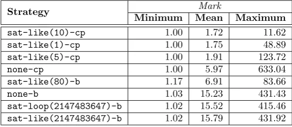
7.4 Strategy Performance - Time . . . 42
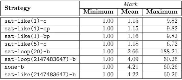
7.5 Strategy Performance - Peak Size . . . 45
7.6 Conclusion . . . 47
8 Classifier Evaluation 48 8.1 Training Data . . . 48
8.2 Metrics Selection . . . 49
8.3 Classification Algorithm Selection . . . 49
8.4 Results - Metrics . . . 51
8.5 Results - Appropriateness . . . 52
9 Feature Relevance 55
9.1 Approach . . . 55
9.2 Results - Time . . . 56
9.3 Results - Peak Size . . . 58
9.4 Conclusion . . . 61
10 Conclusion And Future Work 63 References 65 List of Figures 69 List of Tables 70 A Metrics Using Micro-averaging 71 A.1 Definitions . . . 71
A.2 Recallµ equals Precisionµ . . . 72
A.3 F-Measureµ equals Recallµ. . . 72
A.4 Accuracyµ equalsRecallµ . . . 72
A.5 Remarks . . . 73
B Strategy Evaluation - Data 74 B.1 Capability . . . 74
B.2 Performance - Time . . . 75
B.3 Performance - Peak Size . . . 79
C Classifier Evaluation - Data 83 C.1 Appropriateness - Time . . . 83
C.2 Appropriateness - Peak Size . . . 86
D Reproducibility 91 D.1 Remarks . . . 91
D.2 Data Collection . . . 91
D.2.1 Preparing Environment . . . 91
D.2.2 Defining Experiments . . . 92
D.2.3 Running Experiments . . . 92
D.3 Data Analysis . . . 93
D.3.1 Parsing Data . . . 93
D.3.2 Refining Data . . . 94
D.3.3 Strategy evaluation . . . 95
D.4 Classifiers . . . 95
D.4.1 Training Data Creation . . . 95
D.4.2 Classifier Creation And Evaluation . . . 95
1
Introduction
This chapter gives an introduction to the research described in this thesis. Section 1.1 sketches the context in which the research is performed and provides motivation for this research. Section 1.2 formulated the problems this research aims to solve and a possible solution. Section 1.2 further describes how the solution is accomplished by listing the goals of this research. Section 1.3 describes how the research is performed in order to achieve the stated goals. This chapter concludes with section 1.4 which gives an overview of the structure of this report.
1.1
Background
During creation of programs and software is almost impossible to create a fault free product. As result, the product may behave worse than intended due to the presence of programming errors. An obvious way to increase the quality of a software product is to discover and fix programming errors. Testing is a popular method to discover errors. However, testing can be time consuming and is limited to indicating errors and cannot guarantee the absence of errors. More advanced techniques are needed when one wants to guarantee the presence or absence of certain properties. Formal verification offers the methods and tools to guarantee properties of programs.
Formal verification is the field where one proves or disproves whether a program satisfies some specified formal behavior. This is a powerful method to indicate that a program satisfies certain desirable properties and does not have certain undesirable properties. When a property cannot be proved, this may indicate that the program is lacking some desirable behavior. That information can be used to improve the program, leading to higher quality software.
Formal verification is not limited to evaluation of software. It is also a powerful tool to verify hardware, specifications of protocols or designs. The program, hardware, protocol or design may be too complex to verify directly. It is common that a specification is made, capturing the most important behavior of the object to be verified. The specification of the object where formal verification is applied to is called the model.
1.1.1 Verification Methods
and location of errors and fixing incorrect models.
The second formal verification method offers a solution for the two problems with theorem proving. State space methods analyze models by constructing the state space of the behavior of a model. The state space basically informs which states are possible in a given model. The questions for the object under verification are answered using the state space. Globally, the state space methods can be grouped in two categories: explicit methods and symbolic methods. The methods differ in how the states are stored during the exploration of a model. Explicit methods allocate a fixed amount of memory per state. Symbolic methods use binary decision diagrams (BDD’s) or a variant of BDD’s to store the states.
The construction and analysis of a state space can mostly be done automatically. Hence, state space methods can be applied by less trained personnel and is less time consuming than theorem proving. State space tools are better in providing the location of errors, because they are based on the behavior. There is, however, a major drawback of the state space methods: the state space explosion problem [41]. Informally, this means that when the size of a model grows linearly, the size of its state space grows exponentially. As result, the state space of most models are too huge to analyze.
1.1.2 State Space Methods In Practice
Despite the state space explosion problem, state space methods are still useful in practice. Many measures have been developed in order to cope with large state spaces, including partial order reduction, abstraction and limiting to specific verification questions [8, 41]. On the other hand, much research is performed on techniques to traverse the state space efficiently. A wide range of tools exist which implement one or multiple techniques to perform state space analysis. As result, a user has many options to apply state space methods on his or her models. In this thesis we will call such a option a strategy. In the most abstract form, a strategy describes how a state space method is applied on a model. Practically, a strategy could be a setting of tool in combination with the algorithms selected of that tool.
This wide variety of strategies raises two problems. An advantage of state space methods is that the tools are mostly automated, which can be applied by less trained personnel. Because of all the options, users has to learn more about the methods and tools, before they can apply them to their models. Moreover, the variety of models is huge. This makes it almost impossible to learn good strategies beforehand. By experience, or by trial and error, one can learn good strategies. This requires more specifically trained personnel for formal verification.
be verified. This is not a desirable property.
Ideally, the user should not be bothered with the details of the strategy when a state space method is applied. In the best case, the user only has to select the model and the verification question to be solved. Any tool implementing state space methods should determine how to solve the verification question efficiently by itself, without user intervention. As result, the available resources can be utilized optimally to verify models, without almost any user intervention.
1.2
Goals
As result of the state space explosion problem, state space methods lacks a form of simplicity due to the many options to tackle large state spaces. This makes state space methods less automated and requires more specifically trained personnel for formal verification. When a bad set of options is selected, state space methods can waste resources or may be unable to solve certain models, which could be verified with another strategy.
Instead of providing the user a large scale of options, it would be convenient to let model checking tools decide which strategy should be applied on the models to be verified. The tools themself could determine a suitable strategy in order to optimally verify a model using the available resources. As result, more and larger models can be verified using less trained personnel. This research investigates whether is it attainable for a model checking tool to determine a suitable strategy based on the properties of a model.
It is mainly unknown which strategies works well in practice. Therefore, we want to investigate how the state space exploration is affected by different strategies. This research investigates whether a fixed strategy should be enforced by a model checking tool or whether a model checking tool should dynamically predict a suitable strategy based on the properties of the given model.
Assuming that there exists no fixed strategy which optimally solves the wide variety of models, it needs to be established whether the model itself provides sufficient information to predict a suitable strategy. This research investigates whether a specified set of properties of a model can predict an appropriate strategy. Furthermore, it is investigated whether each property provides any useful information to predict a suitable strategy.
1.3
Approach
The test data was also used to extract a list with the best strategy per model. This list was used to investigate whether properties of a model can predict an appropriate strategy. If such a prediction is possible, this can be implemented in existing tools to improve state space exploration.
Since the relation between the properties of a model and the best strategy was expected to be nontrivial, machine learning techniques were used to capture the relation between a model and its best strategy. The test data was used to train multiple classifiers. Any of the created classifiers can be used as prediction module within an existing tool.
The classifiers were created using all selected properties of a model. In order to investigate whether each property provides any information, variations of the classifiers were made with different subset of features. These variations provide insight in which properties are relevant to consider and which properties can be ignored for predicting an appropriate strategy.
1.4
Structure Of Thesis
In this chapter, the context of our research is given. Chapter 2 discusses the model checking tool LTSmin used during our research. Chapter 3 gives an introduction to machine learning. In chapter 3, the creation and evaluation of classifiers in general is discussed. Chapter 4 examines existing work related to our research.
Chapter 5 and 6 discuss the research method. The questions on which this research is based are discussed in chapter 5. The method itself is covered in chapter 6 .
Chapters 7, 8 and 9 discuss the results obtained during our research. Chapter 7 discusses the relevant observations obtained during the evaluation of the selected strategies. Chapter 8 evaluates the created classifiers and discusses the performance of the classifiers with respect to metrics and to the performance of the selected strategies. Variations of the classifiers were created by using subsets of features. The results show the relevance of each feature. These results are discussed in chapter 9.
2
Preliminaries - LTSmin
This chapter gives an overview of the LTSmin toolset which is used during this research. Section 2.1 gives an overview of the tool. Sections 2.2, 2.3 and 2.4 describe the three layers which can be distinguished in the architecture of
LTSmin. Section 2.5 provides a summary of LTSmin.
2.1
Tool Overview
The LTSmin toolset is a high performance model checker [16]. Its modular nature allows to analyze models specified in various languages by various analysis algorithms. This is possible because of the presence of a common interface called
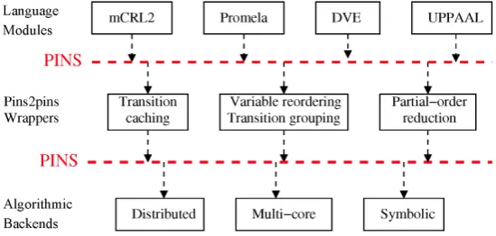
PINS. The architecture of LTSminconsists of three layers, where each layer
[image:11.595.158.433.419.550.2]is connected via the PINS interface, see Figure 1. The PINS interface is an implicit state space definition of a model and is used to exchange information between the different modules inLTSmin. It should at least provide the initial state, the partitioned transition function and a labeling function of a model, which together describe a transition system, hence describing a state space. On top of this basic information different extensions are possible [16, 21]. These extensions can be utilized to exchange information about dependencies in the model, which can be exploited to improve model checking. Within our research the dependency matrix of a model, provided by the PINS interface, is used. The dependency matrix defines which transition groups affect which variables in a model.
Figure 1: Schematic overview of the architecture of LTSmin.
2.2
Front-end Modules
The front-end modules specify how various languages should be mapped to the
PINS interface. This allows users to use the various analysis algorithms of
LTSminnot supported in their native tools, without changing the specification language [3]. Currently, LTSmin supports the languages DVE, Promela,
their own custom model specifications inCby implementing thePINSinterface [16].
2.3
Wrapper Modules
The intermediate layer offers various tools to optimize the performance, reduce the state space or verify certain properties. Because they only rely on the model definition by the PINS interface, they can be applied on any model. Currently, it is possible to verify properties specified in LTL and µ-calculus [16]. LTSminoffers partial order reduction [41] for the explicit back-ends and variable reordering for the symbolic back-end. These modules can be enabled to improve state space exploration.
2.4
Back-end Modules
Model checking can be done by storing the states either explicit or symbolically.
LTSminsupports both options. Furthermore, the toolset supports verification using multiple cores or distributed systems [16, 18]. Each back-end has its options to specify which algorithm or package it should use and with which configuration. These options allow the user to select specific algorithms or to specify how many resources are used by LTSmin.
2.5
Summary
The LTSmin toolset is a high performance model checker which offer various verification methods for multiple different specification languages. LTSmin
3
Preliminaries - Machine Learning
This chapter gives an overview of machine learning and introduces the metrics used for evaluating the created classifiers in our research. Section 3.1 gives a overview of machine learning and identifies the different subfields within machine learning.
In our research, machine learning techniques are used to predict a strategy given a set of features of a model. More specifically, the goal is to predict which strategy within a finite set of strategies is the most appropriate for a given set of features. The prediction of a strategy is a classification problem. Section 3.2 focuses on the general approach to tackle a classification problem by creating a classifier. Section 3.3 demonstrates three techniques which can be used to train a classifier. Section 3.4, 3.5 and 3.6 discuss metrics to evaluate classifiers. Section 3.4 defines the basic metrics for classification problem consisting of two different classes. These basic metrics are used in section 3.5 to define metrics for classification problems consisting of three or more classes. Section 3.6 discusses how different types of misclassification can be taken into account by specifying cost or reward per classification of an instance.
3.1
Overview
Machine learning is a subfield in computer science which is concerned with giving a computer the ability to learn. Computers are utilized by giving them a set of instructions to execute in order to perform a task. The set of instructions is usually given by a script or a program, which explicitly describes the steps the computer has to execute. Machine learning deals with giving the computer the ability to learn the steps from data instead of giving the steps explicitly to them. This approach is often utilized for more complex programming tasks where is it infeasible to describe and cover the problem by giving the instructions directly, such as handwriting recognition or image processing. Instead the computer is given an algorithm to learn the relation between the input data and the tasks it has to perform. In the case of handwriting recognition, the input data may be a written text and the task may be to recognize the individual characters of the text.
Within the field of machine learning three subfields can be globally distinguished: supervised, unsupervised and reinforcement learning [11, 15, 23]. These subfields are briefly addressed in sections 3.1.1, 3.1.2 and 3.1.3 respectively.
3.1.1 Supervised Learning
Within a classification problem a finite number of classes are defined. The computer is given a dataset of input and class couples. The goal of the computer is to determine the class of new, unseen input. Any program that is able to predict a class based on the input is called a classifier. Actually, any program with the purpose to assign a class to an instance of a classification problem is considered a classifier. When a classifier has to chose between two classes the classifier is a binary classifier. Otherwise, the classifier is called a multiclass classifier.
3.1.2 Unsupervised Learning
Unsupervised learning differs from supervised learning with respect to the provided data to the computer. Instead of providing both input and expected output data, in unsupervised learning only the input data is provided. The tasks of the computer is to discover patterns in the input data [11]. These types of techniques are useful in data mining, where the focus is on discovering relations, but the prediction capabilities of the model are less important.
3.1.3 Reinforcement Learning
The third subfield in machine learning is reinforcement learning. In reinforcement learning the computer has to perform its task in a dynamic environment [15]. The computer has to do actions based on the current state it perceives from the environment. Each action is rewarded with a reinforcement value. The reinforcement value is used by the computer to decide whether its action was good or bad. The goal of the computer is to maximize the reinforcement value over a long period of time. Via trial and error, the computer learns to operate in its environment.
3.2
Classifier Creation
There exists a wide variety of classification problems. In general, one wants to determine the class of a large number of instances. The idea is to create a classifier which is able to determine the class of these instances. As mentioned in section 3.1.1, any program which determines a class for an instance is considered a classifier. Two examples of classifiers are given in section 3.4.3 and 3.5.4. Within machine learning the classifier is created by offering training data, instead of explicitly describing when a given instance belongs to a certain class. After the classifier is trained it is able to predict the classes for new instances. In general, a classification problem is solved using the following steps [23]:
1. Defining the problem. Firstly, it needs to be established which problem the classifier to be created has to solve. The main goal is to specify the instances of the problem and the corresponding classes.
3. Training a classifier. After collecting the data, a training method is selected how the classifier should learn. This method is called the classification algorithm. The classifier is trained with the collected data. After training, the model is ready to determine classes for new, unseen instances.
4. Evaluating the classifier. The classifier may be evaluated in order to determine its quality. The evaluation can be performed on both seen and unseen data. In the last case, a fraction of the data collected during the first step should not be used for training the classifier. During this phase, one can evaluate whether the amount training data is sufficient for the classifier to determine classes for other instances. If the performance of a classifier is poor, a new classifier can be created using other or more features such that the classifier can operate more accurately.
5. Utilizing the classifier. When a classifier with a desirable quality is created, the classifier can be used to solve the classification problem it was designed for.
For a given problem it is common that multiple classifiers are created and evaluated. A common option is that 70% of the data is used for training, while the remaining 30% is used for evaluation. This allows the user to select the most appropriate classification algorithm or to investigate the selection of features. It is possible that this approach reveals which technique is the most useful for the problem at hand. Based on the results a new classifier may be created which uses the entire collected dataset. That classifier will be used to solve the classification problem.
3.3
Classification Algorithms
Different algorithms exists to train a classifier. This section briefly covers three training methods. These methods do not completely cover the available classification algorithms, but give an idea how certain methods train classifiers.
3.3.1 Decision Trees
Decision trees are based on the tree data structure. Each node in a decision tree is a question which can be either true or false for an instance. Each leaf node contains one of the possible classes. The tree is built using the training data. For new instances the tree is traversed to determine the class. Starting with the root node, the questions of the nodes are answered for the given instance and the corresponding branch is taken. The questions are answered until a leaf node is reached. The class of the encountered leaf node is the predicted class for the given instance.
3.3.2 K-Nearest Neighbors
instance, the k-nearest neighbors method finds theknearest points with respect to the location of the instance in the defined space. The classes of these nearest points are used to determined the class of the new instance by majority vote.
3.3.3 Support Vector Machines
Support vector machines like k-nearest neighbor also treat the instances as points in a space. Support vector machines try to define hyperplanes which separates the points into their corresponding classes based on the training data. When given a new point, support vector machines check between which hyperplanes the point is located. That outcome decides which class is predicted for the given instance.
3.4
Binary Classifier Evaluation
In machine learning, classifiers are evaluated by examining multiple inputs and comparing the predicted class with the expected class. In general, one can say that the quality of the created classifier depends how closely the predicted classes matches the expected classes. Within machine learning different metrics did arise to formally capture this notion in order to provide information of the quality of classifiers. This section covers the evaluation of binary classifiers.
3.4.1 2×2 Confusion Matrix
The performance of a binary classifier can be recorded using a confusion matrix [24, 39]. A confusion matrix is a special type of contingency table where the rows matches the columns. For a binary classifier the confusion matrix is a 2×2 matrix as depicted in Table 1.
Predicted class
Positive Negative
Actual class Positive True Positives False Negatives
[image:16.595.156.436.472.526.2]Negative False Positives True Negatives
Table 1: 2×2 Confusion matrix for a binary classification problem.
The possible classes of any binary classification problem are usuallyPositiveand
Negative. Any definition of two classes can be rewritten into these classes. The confusion matrix summarizes which classes for the test instances are predicted. The rows indicate the classes of the instances in the validation data. The columns indicate the predicted class by the binary classifier. The entries in the confusion matrix count how many instances from the class specified by the row are predicted as from the class specified by the column.
3.4.2 Metrics
TP =True Positives; the number of instances correctly classified asPositive.
FN =False Negatives; the of number of instances erroneously classified as
Negative, but arePositive.
FP = False Positives; the number of instances erroneously classified as
Positive, but areNegative.
TN = True Negatives; the number of instances correctly classified as
Negative.
The metrics for binary classifiers are constructed using these four values. The following metrics exist:
Recall = TP
TP+FN Precision = TP
TP+FP Specificity = TN
TN+FP
Accuracy = TP+TN
TP+FN +FP+TN
F-Measure = (β
2+ 1)·TP
(β2+ 1)·TP+β2·FN +FP
The minimum value for any of these metrics is 0, indicating that all instances are misclassified. The maximum value is 1, which corresponds to that all instances are correctly classified. Any classifier that randomly classifies instances will get 0.5 for each metric1.
Recall indicates which fraction of thePositive instances is correctly classified. This can be interpreted how well the classifier recognizes thePositive instances. When a classifier classifies all instances to Positive, Recall is maximum. In order to distinguish this behavior Precision can be used to verify how likely a classifier will classify an instance to Positive. Specificity resembles the Recall
metric for Negative instances.
Accuracy defines the fraction of instances that is correctly classified. This is useful for obtaining a general idea of the performance, but it does not state how well each class is recognized by the classifier.
F-Measure combines Precision and Recall to evaluate the performance of a binary classifier. Both metrics are weighted allowing the user to prioritize either metric. The weight for Precision and Recall is 1 and β2 respectively. These weights are derived from Van Rijsenberg’s effectiveness measure [43].
Besides the five binary metrics discussed above, other metrics exist for binary
classifiers. Examples include AUC [13], Cohen0s Kappa [9], Matthews Correlation Coefficient [20] and Youden0s J Statistic [45]. These metrics capture the performance of classifying instances of both classes, while the metrics
Recall, Precision and F-Measure focus on the Positive instances and do not take the True Negatives into account. This is useful when both classes are of equal importance. However a drawback ofAUC,Cohen0s Kappa,Matthews Correlation CoefficientandYouden0s J Statisticis that these metrics are solely defined for binary classifiers [19].
3.4.3 Example - Spam Filter
In order to demonstrate the metrics given in the previous section, an example is discussed. The example describes the evaluation of a spam filter. A spam filter should mark messages as spam or not-spam. The creation of a spam filter is based on the ability to classify whether a message is spam or not. Whether a message is spam is a binary classification problem, because there are two classes: spam messages and non-spam messages.
Suppose we collected a dataset of 300 messages. A spam filter is created by training a classifier using 200 instances of our data. The remaining 100 instances are used to evaluate the spam filter. 40 of the 100 messages are assumed to be spam, while the other 60 messages are considered non-spam. The predicted classes for these instances by the created classifier are listed in the confusion matrix given in Table 2. It is assumed thatPositiveis the class of spam messages andNegative is the class of non-spam messages.
Predicted class
Positive Negative
Actual class Positive 36 4
Negative 11 49
Table 2: A 2×2 confusion matrix for a spam filter. Positive is interpretted as being a spam message, while Negative is considered as being a non-spam message.
Using the confusion matrix the following values are defined:
TP = 36
FN = 4
FP = 11
TN = 49
Then the following values are assigned to the metrics of this classifier:
Recall = 0.900
Precision = 0.766
Accuracy = 0.850
F-Measure = 0.828 (forβ= 1)
Based on these values, the following conclusions can be derived. Considering
Recall, the classifier is able to recognize 90% of the spam messages. However, of all messages that were classified as spam, only 77% was actually a spam message based on the value forPrecision. Specificityindicates that 82% of the non-spam messages are correctly recognized, while the other 18% is erroneously classified as spam. Lastly, the value for Accuracy shows that 85% of all messages was correctly classified.
3.5
Multiclass Classifier Evaluation
The evaluation of multiclass classifiers does not differ much from the evaluation of binary classifiers. However, the evaluation metrics are solely defined using the metrics for binary classifiers [37]. Therefore, the evaluation of multiclass classifiers is discussed separately.
3.5.1 n×n Confusion Matrix
The performance of a multiclass classifier can be recorded using a confusion matrix [24]. Instead of using a 2×2 confusion matrix, an×nconfusion matrix is used, wherenequals the number of classes of the corresponding classification problem. The rows list the different classes and the columns list the predicted classes. Each value in the confusion matrix indicates how many instances of classxare recognized as classy. These values can be used to check how many instances are correctly classified and how many instances are confused by the classifier for being in a different class. The general form of a confusion matrix is given in Table 3.
Predicted class
Class 1 Class 2 ... Class n
Actual class
Class 1 Correctly classified 1’s
1’s confused for 2’s
... 1’s confused forn’s
Class 2 2’s confused for 1’s
Correctly classified 2’s
... 2’s confused forn’s
... ... ... ...
Class n n’s confused for 1’s
n’s confused for 2’s
... Correctly classified n’s
Table 3: n×n Confusion matrix for a classification problem consisting of n
classes.
3.5.2 Transformation To 2×2 Confusion Matrix
Anyn×nconfusion matrix can be transformed to another confusion matrix of
Specifically, one transformation is used, which separates the classes in a one versus rest manner. This transformation transforms a n×nconfusion matrix to a 2×2 confusion matrix. The Positive class consists of one specific class, while theNegativeclass consists of the remainingn−1 classes. The values in the resulting 2×2 confusion matrix are a defined by combining the individual entries of the givenn×nmatrix based on the new classes. This transformation is called
Flatteniin this thesis, whereidefines the class which becomes thePositiveclass.
More formally, Flatteni is a function on a n×n matrix A, which returns a
2×2 confusion matrixB. The entries of B are defined as follows:
TP =Aii
FN =
i−1
X
k=1
Aik+ n
X
k=i+1
Aik
FP =
i−1
X
k=1
Aki+ n
X
k=i+1
Aki
TN =
i−1
X
k=1
i−1
X
m=1
Akm+ n
X
m=i+1
Akm
!
+
n
X
k=i+1
i−1
X
m=1
Akm+ n
X
m=i+1
Akm
!
An example of this transformation is given in section 3.5.4.
3.5.3 Metrics
The metrics for multiclass classifiers are based on the metrics for binary classifiers [37]. The metrics are defined using the entries of an×n confusion matrix. It is assumed that there are n classes named 1, 2, ..., n. The performance of a multiclass classifier is given by a n×n confusion matrix A. Firstly, for each classithe confusion matrixBiis determined using theFlatteni transformation
as defined in the previous section. The following definitions are used, assuming
Bi=Flatteni(A):
TPi =True Positives ofBi FNi =False Negatives ofBi FPi =False Positives ofBi TNi =True Negatives ofBi
Each metric defined for binary classifiers can be applied on the confusion matrices Bi in order to determine the performance of the multiclass classifier
per class. The overall performance of the multiclass classifier can be determined in two ways: macro-averaging or micro-averaging the values for a metric for the confusion matrices Bi [33, 40, 44]. With macro-averaging each class equally
The metrics using macro-averaging [37] are defined as:
RecallM =
1
n·
X
i
TPi
TPi+FNi
PrecisionM =
1
n·
X
i
TPi
TPi+FPi
AccuracyM =
1
n·
X
i
TPi+TNi
TPi+FNi+FPi+TNi
F-MeasureM =
(β2+ 1)·Precision
M·RecallM
β2·Precision
M+RecallM
The metrics using micro-averaging [37] are defined as:
Recallµ =
P
iTPi
P
i(TPi+FNi)
Precisionµ =
P
iTPi
P
i(TPi+FPi)
F-Measureµ =
(β2+ 1)·Precision
µ·Recallµ
β2·Precision
µ+Recallµ
Interestingly, Recallµ, Precisionµ andF-Measureµ will give the same value for
any confusion matrix (see Appendix A). This metric resembles the formula for Accuracy and can be considered as Accuracyµ. Accuracyµ indicates like Accuracy which fraction of the models is correctly classified. Using Aij to
denote the value in theith row andjth column inA,Accuracyµ is defined as:
Accuracyµ =
P
iAii
P
i
P
jAij
Like the binary variants, the minimum value for all metrics listed above is 0. A value of 0 indicates that all instances are misclassified. When all instances are correctly classified, each metric attains the maximum value of 1.
3.5.4 Example - Simple Handwriting Recognition
This section demonstrates how the metrics are determined for a multiclass classifier. The evaluation of a simple handwriting recognition system is discussed. The purpose of such a system is to determine which word or character is written given by an image. It is assumed that the simple handwriting recognition system examines individual characters. The goal is to determine whether the character is a letter, a digit or a punctuation mark. The evaluation of the simple handwriting recognition system is given using a 3×3 confusion matrix as given in Table 4.
For each class, a 2×2 confusion matrix is determined using the transformation
Predicted class
Letter Digit Punctuation
Actual class
Letter 37 13 2
Digit 21 56 8
Punctuation 5 0 42
Table 4: A 3×3 confusion matrix for a simple handwriting recognition system. Confusion matrix
FlattenLetter FlattenDigit FlattenPunctuation
Value
TPi 37 56 42
FNi 15 29 5
FPi 26 13 10
TNi 106 86 127
Table 5: 2×2 confusion matrices derived from Table 4.
listed in Table 5.
The values in the 2×2 confusion matrices give the following values for the metrics for the simple handwriting recognition system:
RecallM = 0.755
PrecisionM = 0.736
AccuracyM = 0.822
F-MeasureM = 0.745 (forβ= 1)
Recallµ = 0.734 Precisionµ = 0.734
F-Measureµ = 0.734 (for any real constantβ) Accuracyµ = 0.734
3.6
Metrics For Cost-sensitive Classifiers
For some classification problems the classification of each instance is linked to a reward or cost [10, 12]. When an instance is correctly classified there is a reward (or negative cost) and when an instance is incorrectly classified there is a cost (or negative reward). This cost may depend on which predicted class is chosen for a certain class. For this type of classifiers the total expected reward or cost is more important than the number of instances correctly classified.
3.6.1 Metrics
The concept of classifying instances is paired with cost or reward, can be formally described. Given a confusion matrix A each entry has a weight Wij
metricCostcan be defined as sum of the individual classification costs. Likewise,
Rewardcan be defined as the inverse ofCost. A cost-sensitive classifier performs better when the cost is lower or the reward higher. These metrics defined as:
Cost =P
i
P
jWij ·Aij
Wij ≤0 if i=j
Wij ≥0 if i6=j
Reward =P
i
P
jWij·Aij
Wij ≥0 if i=j
Wij ≤0 if i6=j
Unlike the metrics examined so far, the metricsCost andRewarddo not have a minimum or maximum value. Both the minimum and maximum value depend on the number of instances per class in the validation data and the weights
Wij. Nevertheless, these metrics can be used to compare the classifier with a
predefined threshold or with another classifier evaluated with the same validation data.
3.6.2 Example - Comparing Spam Filters
Spam filters can be used to automatically clean inboxes by removing the messages which are marked as spam. This can be convenient for the user because one does not have to deal with the messages marked as spam. However, is unfortunate when non-spam messages are deleted because the spam filter marked these messages as spam. The user may miss fundamental information contained in these messages.
Suppose there are two spam filters available, whose performance is given by confusion matrices depicted in Table 6 and 7 respectively. Further, it is assumed that misclassifying a non-spam message is five times worse than misclassifying a spam message. Then the weights2 W are expressed by the matrix
0 1 5 0
.
Predicted class
Spam Non-spam
Actual class Spam 48 2
[image:23.595.185.409.493.546.2]Non-spam 8 42
Table 6: A 2×2 confusion matrix for spam filter option A.
Predicted class
Spam Non-spam
Actual class Spam 36 14
[image:23.595.179.407.587.641.2]Non-spam 1 49
Table 7: A 2×2 confusion matrix for spam filter option B.
Although classifier option A is more accurate than classifier option B, the cost of using classifier option A is 42 and the cost of using classifier option B is only 19.
2It is assumed that determining the correct class for a message induces no cost. Therefore,
4
Related Work
This chapter discusses the work related to our research. Section 4.1 shows that the use of symbolic state space methods is necessary but has limitations too. Section 4.2 discusses different proposed methods to improve symbolic state space methods. To our best knowledge, using the features of a model to predict a strategy is a fairly new concept to improve state space exploration. Section 4.3 discusses work related to strategy prediction.
4.1
Symbolic State Space Methods
State space methods rely on examining all reachable states for a given model. The process of discovering the reachable states is called the state space exploration. During state space exploration the discovered states can be either stored explicitly or symbolically.
When the states are stored explicitly, each discovered state is stored in memory, occupying a specific amount of memory. This approach is not suitable for large state spaces. Lets assume that a given model has over 1020reachable states and each state can be stored in 128 bits. Without overhead, this approach will take over 1.6 zettabyte3 of memory. This amount of memory is simply too large for any computer and therefore the use of explicit state space methods is limited to smaller state spaces.
Symbolic state space methods are able to deal with large state spaces [6]. Symbolic state space methods store the discovered states in a Binary Decision Diagram (BDD) or a variant of BDDs. Unfortunately, symbolic state space methods are limited by time and memory too [8]. On top of that, there is no clear relation between the number of states stored and the size of the BDD [32]. During state space exploration the size of the BDD may be much larger than the final BDD describing the entire state space. The largest size encountered during exploration is called the peak size of de BDD. The peak size is often reached midway during the state space exploration. The peak size may be hundreds or thousands of times larger than final size of the BDD, placing a high demand on resources [8]. Therefore, it is important that during the exploration of the state space, the size of the BDD is kept as small as possible in order to utilize the available resources the most efficient.
4.2
Improvements Of State Space Methods
Due to the state space explosion problem [41] it may be unfeasible to directly apply either explicit or symbolic methods on given models. Since the introduction of state space methods, much research is performed to enhance state space methods, allowing to investigate more models and larger state spaces. This section gives an overview of improvements which are related to our research, which aims to improve state space methods.
4.2.1 BDD Construction
Symbolic state space methods rely on BDDs. The way the BDD is constructed affects the performance of a state space method. The peak size of the BDD determines the amount of resources needed [8]. Since the peak size may be significantly larger than the final size of the BDD, it is important that the size of the BDD is kept as small as possible. Maintaining a small BDD allows to explore larger state spaces.
The size of the BDD depends on how the variables in the BDD are ordered. The variables can be reordered in order to reduce the size of the BDD, but determining this order is a NP-complete problem [4]. Therefore it is not feasible to perform variable reordering according to the best variable order during state space exploration.
Since it is not feasible to maintain the best variable ordering during exploration, other methods were proposed to reduce the peak size of a BDD. Some methods aim to find a good variable ordering beforehand [14, 22, 35] or try to maintain a good ordering during exploration [31].
4.2.2 Partitioning Of Transitions
Another improvement is to divide the transitions of the model into groups [5]. This method is able to verify models with 1050and 10120states and is required to investigate models with large state spaces. This idea was applied in the
PINS interface of LTSmin[3]. The partition was improved by distinguishing
read and write-dependencies and it was shown that a significant improvement can be achieved [21].
4.2.3 State Space Traversal Techniques
The construction of BDDs also depends on order of the states discovered during exploration, so the way the state space is traversed influences the size of the BDD. As result, different traversal algorithms were proposed.
The classical breadth-first-search (BFS) is a suitable traversal algorithm for state space exploration. An alternative traversal algorithm called chaining was proposed by [30]. This traversal technique was applied on Petri Nets and was found two orders of magnitude faster than regularBFS. However, they admitted that this statement is not verified on larger models.
Ciardo et al [8] gave a variation of both BFS and chaining where all states were used instead of only the previous discovered states. Their results showed that these variations were overall slightly better, but for some models they worsen the amount of resources needed for the state space exploration. They showed that chaining is marginally better thanBFS. However they only presented these results for five selected models.
of concurrent systems and showed that in most cases an improvement can be achieved. Still, chaining was found to be a good alternative.
4.2.4 Saturation
Saturation is another method to greatly reduce the peak size of a BDD [7, 8]. The general idea is that only transitions at a certain level in the BDD are fired. When all transitions are applied, that level is saturated and a higher level is examined. By saturating levels in the BDD, the size of the BDD is kept small. It was reported that this method may achieve several orders of magnitude better performance [7].
4.3
Strategy Prediction
5
Research Questions
This chapter discusses the research questions of this project. The research questions specify which problems the research aims to solve in order to reach the goal specified in chapter 1, namely letting the model checking tools itself decide which strategy is suitable for a given model. The research is formulated using one main question described in section 5.1. The main question is subdivided in three research questions which are described in section 5.2, 5.3 and 5.4. Section 5.5 summarizes the research questions.
5.1
Main Question
As mentioned in chapter 1, state space methods may consume many resources due to the state space explosion problem [41]. Currently many different solutions are proposed to tackle the state space explosion problem. The user is provided multiple strategies to solve its models. Because of the wide variety of models and options, it may be hard for the user to select an appropriate strategy. Selecting an inappropriate strategy may lead to a waste of resources or that the model checking tool is unable to answer the given verification questions.
Therefore, the model checking tools itself, instead of the users, should decide which strategy should be applied on a given model. This research investigates whether it is possible for a model checking tool to select an appropriate strategy using only the information presented in the given model. The pieces of information embedded in a model are called the features of a model in this report. Since most verification questions are based on the state space of a model [41], the problem of verifying a model is refined to the problem of determining the state space of a model. This leads to the following main question:
To what extent can the features of a model be used to predict an appropriate strategy in order to improve state space exploration?
It is not necessary to come up with the absolute best strategy currently available. It is sufficient to find a strategy which performs almost as good as the best strategy given a specific model.
This main question is answered using three research questions specified in the remaining of this chapter.
5.2
Research Question 1
Because of the wide varieties in strategies and models, it is unknown how well the strategies perform on different models. This leads to the first research question:
How does the strategy influence the state space exploration of a model?
differences between multiple strategies for a model. If the differences are negligible, any strategy can be selected and the features of the model does not matter.
On the other hand, we examined whether there exists a superior strategy. A superior strategy is a strategy which performs better than any other strategy for almost all models. If any superior strategy exists, that superior strategy should be selected without even considering the features of the models.
5.3
Research Question 2
Assuming the selection of the strategy significantly influences the state space exploration, a best strategy can be selected per model. We investigated how the features of the model relates to its best strategy. This investigation is captured by the second research question:
Which features are relevant to consider when predicting a strategy for a model?
The answer on this question reveals which features are relevant to consider and which features does not provide any helpful information for selecting an appropriate strategy. This information should be exploited by the model checking tools such that during the strategy selection the relevant features are considered and the redundant features are ignored.
5.4
Research Question 3
Lastly, we investigated whether the features provide sufficient information to determine an appropriate strategy. The last research question states whether it is possible to predict an appropiate strategy using the features of a model:
To what extent can we make a prediction of an appropriate strategy given the features of a model?
We checked whether it is possible to determine an appropriate strategy given the features of a model. Since the predicted strategy may depend on multiple features on different domains, it is expected that there does not exists a trivial relation between the features and the best strategy of a model. Therefore, supervised machine learning techniques are used to predict an appropriate strategy given the features of a model.
5.5
Summary
6
Methods
This chapters discusses the methods used in our research. Section 6.1 defines the scope of our research by defining which set of strategies and features are considered. Section 6.2 defines the techniques and materials used in our research. Section 6.3 discusses how the research was performed.
6.1
Scope
The main goal of this research is to investigate to what extent features of a model can be used to predict a strategy. A strategy is defined as any way in which a state space method is applied to solve verification questions. In chapter 5 it was mentioned that the verification questions are confined to the state space exploration. A feature is defined as any property of a model. The terms strategy and feature are too broad to cover in a single research. This sections explains which strategies and features were selected for our research.
6.1.1 Selected Strategies
The number of strategies had to be limited in order to make testing feasible. Considering related work, it can be observed that the traversal method and saturation may significantly influence the state space exploration of a model. Therefore, these two aspects were set variable in a strategy and other aspects of a strategy were fixed. Some of the models which were used for testing, have huge state spaces. The explicit backend of LTSminwas not suitable for these models. Therefore, the symbolic backend of LTSminwas selected.
Four different traversal algorithms were incorporated in our research: bfs, bfs-prev, chain and chain-prev. These algorithms are based on the ones found in [8]. The pseudo code of the algorithms as implemented in LTSminis given in [34]. The traversal algorithms introduced by [38] are not available in
LTSminand were not considered.
LTSmin offers the ability to do saturation, but it differs from the original
method [8, 34]. LTSminoffers multiple options to perform saturation and forces the user to divide the dependency matrix into saturation levels. These levels are defined by a parameter called saturation granularity. The saturation granularity indicates the column width of each level4. The user has to provide a positive integer for this parameter or otherwise a default value of 10 is used.
Multiple different saturation granularities were considered including the extreme values. The minimum value for saturation granularity is 1. The maximum value equals the width of the dependency matrix and any higher value results in the same performance. Since the width of the dependency matrix depends on the model, the maximum value cannot be fixed precisely. Instead the maximum signed integer value (2147483647) was used in order to capture all models.
4In the case the saturation granularity does not divide the width of the dependency matrix,
The values 1, 5, 10, 20, 40, 80 and 2147483647 were selected for saturation granularity.
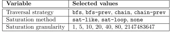
[image:31.595.153.439.279.333.2]Two saturation methods called sat-like and sat-loop were considered. Combining the saturation methods with the selected values for saturation granularity, 14 different saturation strategies were defined. It was also tested how well the models were explored without using saturation (saturation method = none). The saturation granularity does not have any meaning when no satuation is used for exploring the model. Incorporating none as saturation strategy gave an additional strategy. So in total, 15 different saturation strategies were considered. The variables and selected values for strategies are listed in Table 8.
Variable Selected values
Traversal strategy bfs,bfs-prev, chain,chain-prev Saturation method sat-like,sat-loop,none
Saturation granularity 1, 5, 10, 20, 40, 80, 2147483647
Table 8: Selected variables and values for the strategies. Note: saturation granularity was only used when sat-like or sat-loop was selected as saturation method.
The traversal strategy and saturation strategy can be chosen individually for any model. The saturation method defines how the saturation levels are visited, while the traversal strategy defines the method to visit states within a saturation level. So any of the 4 traversal strategies can be combined with any of the 15 saturation strategies, defining 60 different strategies. These 60 strategies are considered during our research.
Besides the variable aspects of the strategies, some aspects were fixed for all strategies. These fixed aspects are listed in Table 9. The reordering strategy was selected from [22] because that reordering strategy had the best overall performance. save-sat-levels is time optimization flag for both sat-like and sat-loop. This flag has no effect when none is selected as saturation method. vsetspecifies the BDD package used. The other aspects enforces that a fixed amount of resources can be utilized for solving a model.
Aspect Selected value
Reorder strategy tg,bs,hf save-sat-levels true
vset lddmc
[image:31.595.205.387.565.669.2]lace-workers 1 ldd-cachesize 26 ldd-tablesize 26 ldd-maxtablesize 26
Table 9: Selected values of fixed aspects for all strategies.
6.1.2 Selected Features
Everything based on the information of the model can be considered a feature. The set of features considered were also limited. SinceLTSminis able to handle different types of models, model specific features were not considered. Model specific features are based on the specification language used to describe the model. The maximum number of arcs leaving any place in a Petri Net or the number of lines in a DVEmodel are examples of model specific features. All features considered in this research were based on features that can be derived for all models LTSmin is able to analyze. This design choice allows that the results produced by this research can be applied to a large variety of specification languages (see section 2.2). Hence, only features which can be derived from the information available in thePINS interface were considered.
Feature Definition
State Vector Length[16] Width of the dependency matrix.
Groups[16]
The number of transition groups. This corresponds to the number of rows in the dependency matrix.
Bandwidth [22] Maximum bandwidth of all rows in the dependency matrix after variable reordering.
Profile [22] Sum of the bandwidth of all rows in the dependency matrix after variable reordering.
Span [22] Sum of the span of all rows in the dependency matrix after variable reordering.
Average Wavefront
Sum of the wavefront of all rows in the dependency matrix after variable reordering divided by the number of rows.
RMS Wavefront
Root mean squared over the wavefront of all rows in the dependency matrix after variable reordering.
Event Span (ES) [22] Sum of the span of all rows in the dependency matrix before variable reordering.
Normalized Event Span (NES) [22]
Normalized version ofEvent Span which allows to compare dependency matrices of different sizes.
Weighted Event
Span (WES) [22] Weighted variant ofEvent Span.
Normalized Weighted Event Span (NWES) [22]
Normalized version ofWeighted Event Span
[image:32.595.126.467.297.629.2]which allows to compare dependency matrices of different sizes.
Table 10: Selected features of the model based on metrics on the dependency matrix.
are based on the following metrics per row [22]:
Bandwidth of a row = Maximum distance of any nonzero entry in a row to the diagonal of the dependency matrix.
Span of a row = Distance between the leftmost and rightmost nonzero entry in a row.
Wavefront of a row = The number of adjacent vertices of all vertices smaller or equal to the vertex corresponding to the row.
6.2
Techniques
This section gives an overview of the models and techniques used during our research. Firstly, the set of models which was used during our research is discussed. Secondly, the tools and programs which were used are listed. The last section gives an overview of the used machines for determining the performance of the selected strategies.
6.2.1 Model Collection
The selected strategies were tested on a large number of models in order to acquire sufficient information. The PNML models of the Model Checking Contest [17] were used. Since LTSmin currently cannot handle colored Petri Nets, only the unfolded Petri Nets were considered. This collection consists of 491 different models. These models are instances of 66 different parameterized Petri Nets5. Furthermore, 293
DVEmodels of theBEEMdatabase6were used
[25]. These models are instances of 56 parameterizedDVEmodels7. So in total 784 different models were used.
6.2.2 Tools And Programs
This section lists the tools and programs used during our research. See section 6.3 for the role of each program.
Overview of the tools and programs: • awkversion 4.0.1
• bashversion 4.3.11(1) • DiViNe[1] version 2.4 • grepversion 2.16
• LTSmin8 A development version was used because there was no stable release which could handlePNML models correctly. LTSminwas build from commitfbc4d4999d06134984f076eed2f0b8523cfb5704.
5This is the collection of theSurpriseandKnownmodels for 2016. The model
DotAndBoxesdoes not offer an unfolded Petri Net variant and is not included in the test cases.
6Available onhttp://paradise.fi.muni.cz/beem/, accessed July 2016. 7All seven instances of the model
train-gatecould not be compiled usingDiVinE. These models are left out of the test cases.
• memtime9
• Pythonversion 2.7.6 • R10version 3.3.1
– ggplot2package version 2.0.0
– plyr package version 1.8.3
– reshape2 package version 1.4.1 • scikit-learn11version 0.17.1
6.2.3 Machines
The computer cluster of the University of Twente was used to measure the performance of the selected strategies. Specifically, 44 machines were used. All machines operate under Ubuntu 14.04 LTS and each machine has 64 GB RAM. The CPU of 32 machines is 2×AMD Opteron 4386, while the CPU of the other 12 machines is 1×AMD Opteron 4386. The AMD Opteron 4386has 8 cores.
6.3
Method
This section explains which actions are performed during our research in order to answer the research questions stated in chapter 5. Firstly, the performance of the selected strategies was determined for the selected models. The resulting data was refined to eliminate errors and remove redundant data. The performance data was investigated in order to establish whether there exists a superior strategy and to what extent the differences between multiple strategies matter. The performance data was used to select the best strategy with respect to time and peak size per model. This data was used to create multiple classifiers. The performance of the classifiers was investigated in order to establish to what extent the features of a model can predict an appropriate strategy.
The technical details of the created scripts and programs are omitted during the discussion of the research method. Appendix D gives insight in the scripts and discusses how the scripts can be utilized to reproduce the results given in this thesis.
6.3.1 Running State Space Exploration Tests
The purpose of our research is to determine to what extent features of a model can predict an appropriate strategy. In order to measure whether a certain predicted strategy is appropriate, the performance of multiple strategies need to be known for a given model. In section 6.1 the strategies and features were selected. The first step consisted of collecting the performance data of the 60 selected strategies for all 784 selected models.
9Available on http://fmt.cs.utwente.nl/tools/scm/memtime.git/, accessed October
2016.
ThePNMLmodels12were extracted from the website of the MCC. The unfolded Petri Nets were separated from the colored Petri Nets using grep. LTSmin cannot handleDVEmodels directly. DiViNe[1] was used to compile theDVE models toDVE2Cformat.
In order to determine the performance of a strategy on a model accurately, multiple performance runs were performed. The performance of LTSmin is slightly variable due to the load of the system where the tool is running on. Therefore, ten performance runs per model and strategy pair were performed. Besides the performance runs per model and strategy pair, a single statistic run was performed. The purpose of this run is to measure the peak size. Enabling the collection of statistics in LTSmin negatively influence the performance. So the statistics were collected in a separate run. Since LTSmin is deterministic, one statistics run per model and strategy pair suffices. In total, eleven runs were performed per model and strategy pair.
For each model, the values for the features ES, NES, WES and NWES were determined in a separate run. The values for the other seven features could already be extracted from the other runs. The features of a model are in independent of the selected strategy. The collection of the values of these four features required an additional 784 runs.
This approach required 518224 runs13. The computer cluster of the University of Twente was used to process this large amount of test cases. An existing bash
script was available which was able to generate test cases and automatically schedule the generated test cases on the cluster. This script was modified in order to run with the collected models and the configurations of LTSmin. The
bash script generated a small script per run. Each small generated script
performed one run with the LTSmin tool. The bash script also generated a scheduler script. The generated scheduler script schedules the small generated scripts on the cluster. This method allowed that batches of test cases could be scheduled and executed on the cluster.
It is known that some PNML models are too complex to be analyzed [17]. Because of the large number of test cases, it was preferred that many test cases could run in parallel. Therefore, each test case acquired one CPU core. Each test case acquired 8 GB of RAM. This amount is sufficient to store the BDD and the model itself. If the run exceeded the amount of memory or took too long to solve, the test case was aborted. The time limited was set to 30 minutes. These constraints were enforced by usingmemtime. Furthermore,memtimerecorded the elapsed time and memory footprint.
6.3.2 Processing Data
The output ofLTSminis plain-text. After running all test cases on the cluster, the output of each run was stored in a txt-file. Due to the large amount of files, it is impossible to analyze those files by hand. 30 files were randomly selected
to identify the possible formats LTSmincould produce. This information was used to create a parser in bash. The programs grep and awk are natural to use to extract information of text and were used extensively by the parser. The parser notified the user if it did not recognize the format of the provided text-file. In this way, new formats were discovered and the parser was updated for those formats. As result, all txt-files were successfully parsed. The results were stored in a csv-file.
The programming languageRwas used for the analysis of the csv-file. Roffers various tools to filter and aggregate data, and it is natural to use for data mining. The packages plyr andreshape2 were used for data compression. The data produced by the parser was not suitable to analyze directly. The data had the following issues:
• Some models are unsolvable for all 60 selected strategies. These models cannot be used, since it is impossible to measure whether the predicted strategy is appropriate for these models. Furthermore, because some models are too large, even the values of some features could not be determined.
• Some models were not solved correctly. For most models the actual or a lower bound of the size of the state space is known. There are 59 models where all selected strategies could not solve the model or produced wrong results. Since these models were solved incorrectly, the performance of the strategies may not reflect the actual effort needed to solve the models correctly. These models were removed from the data.
• The data contains contradicting entries. This was revealed by the size of the calculated state space for a model. The state space is always fixed for a given model, so LTSmin produced faulty results for some models. For some models in combination with a selected saturation granularity of 1, the state space was reported extremely small14, while it is known that the state space is significantly larger.
• The saturation granularity was selected before solving a model. The meaning of saturation granularity depends on the width of the dependency matrix of the model. If the saturation granularity is larger than the state vector length, the strategy does not differ from the equivalent strategy with a saturation granularity of 2147483647. Hence for smaller models, multiple different strategies may collapse in a single strategy, although they are marked as different strategies in the data.
• Due to the multiple runs per model and strategy pair, the information of the performance of a model with respect to a strategy is scattered over the entire csv-file. The performance of a strategy on a model is defined by at least eleven lines.
Before the data was analyzed, the issues mentioned above were addressed. Firstly, all runs of the models which could not be solved correctly by any strategy, were removed. These 59 models were identified by comparing the