Using the Prony Analysis for Assessing Servo Drive Control
Reimund Neugebauer, Ruben Schönherr*, Holger Schlegel
Chemnitz University of Technology, Faculty of Mechanical Engineering, Institute for Machine Tools and Production Processes, Chemnitz, Germany
E-mail:*[email protected]
ReceivedJune 10, 2011; revised July 1, 2011; accepted August 8, 2011
Abstract
The Prony Analysis is already used in different fields of science and industries. The described new approach intends assessing the performance of Servo Drive Control. The basic approach is, that two important dy- namic parameters of closed loop behavior, damping and frequency, are estimated by the Prony method. Hence analyzing a control loop in this way leads to a statement concerning the quality of control and allows comparing different parameter sets. The paper presents results achieved by using this method on a test rig.
Keywords: Servo Drive, Control, Assessment, Monitoring, Prony Method
1. Introduction
Several mathematical approaches proofed to be practical for monitoring functions and assessment purposes in refineries and chemical plants. Therefore, automatic con- troller assessment is a known feature of state-of-the-art process controlling systems. The most common term in literature for these methods is “Control Loop Perform- ance Monitoring” (CLPM).
Observing the controller behaviour of servo drives in a similar way ought to be advantageous for machines in production industries. Due to a raising number of direct drives and lightweight components, controller settings have a growing influence on the overall system behav- iour. Thus, detecting inadequate control characteristics becomes also more important for process reliability. Furthermore, monitoring methods could contribute to the reduction of energy consumption in the drive by auto- matically recognizing aggressively tuned controllers.
The idea of implementing the known methods in drive controllers is the most obvious way in order to benefit from the research in the field of process control moni- toring. However, several differences between the two fields of controlling impede this direct approach. The main drawback results from the different objectives of controlling:
In process industries, control is focused on keeping the controlled variable close to a constant setpoint. Thus disturbance rejection is of major importance. In com- parison to this, drive systems are supposed to follow a dynamically changing setpoint. So, emphasis is placed
on tracking capabilities. The following Table 1 points
out to further differences between process and servo drive control.
Because of these disparate properties, the known methods of CLPM can not easily be implemented into drive systems. Especially the traditional attributes for assessing controller performance like output variance [2] are not suitable for drive systems. This leads to a need for new methods of controller assessment in the field of servo drives.
Servo Drive Control
Appart from some special applications, the cascaded loop structure shown in Figure 1 is the basis of most
controlled (electrical) drive systems [3].
The paper focuses on the velocity feedback control of electrical servo drives because of different reasons. Two should be mentioned here:
Firstly, monitoring of the current control loops behav- iour is not expected to be very useful, because it depends on the well known or measurable parameters inductance and resistance. So automatic tuning is state of the art and leads to feasible results. Furthermore parameters are nearly constant over time, so deterioration of behavior is not expected.
Secondly, the velocity controllers’ behavior limits the achievable dynamics of the position controller. So the velocity control loop is of major importance regarding the drive dynamics.
Table 1. Comparison between process and servo drive control [1].
Process Control Servo Drive Control
Mostly constant setpoint Setpoint trajectory
Optimized for disturbance rejection Tradeoff between disturbance rejection and tracking capabilities
Large time constants (to minutes or hours) Time constants in the dimension of milliseconds
[image:2.595.121.477.94.287.2]Sample time << time constants Sample time and time constants of the same order
Figure 1. Cascaded position control loop either with direct or indirect position sensor.
to the requirements of drive control assessment. Therefore a different value for characterizing control action is chosen.
2. Damping as Benchmark
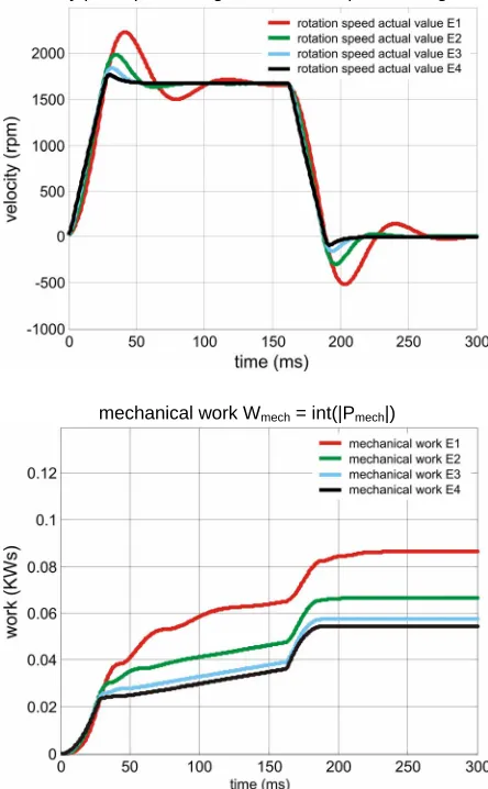
Experiments proofed the influence of velocity controller settings on the energy consumption of the drive (Figure 2).
For this reason, on the one hand, the benchmark should allow the detection of considerable high overshot or os-cillating transition response. On the other hand, sluggish transition behaviour results in loss of dynamics, so this case must also be considered. Assuming a vibratory sec-ond order lag element, the distinction of the two charac-teristics mentioned above can be achieved by the analy-sis of the damping D.
2 2 2 1 K G sT s DTs
(1)
(K: gain; T: time Constant; D: damping)
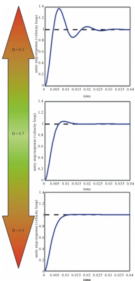
In an initial approximation, the second order lag model fits to the closed velocity control loop. A damping of approximately 0.7 is aspired in most cases [3]. Especially a less damped behavior, which leads to a large overshot and higher energy consumption, should be avoided. A bigger damping causes a loss of dynamics and is there- fore also disadvantageous (Figure 3).
In order to derive a statement about the damping, a sufficiently high excitation of the analyzed system (here the closed velocity control loop) is necessary. Different time domain methods are known to identify the damping of vibratory second order lag systems [1,4]. These meth-ods base chiefly on analyzing the overshot-heights, sometimes combined with detection of zero crossings.
velocity plots: positioning for 5 rotations positive/negative
mechanical work Wmech = int(|Pmech|)
[image:2.595.311.533.322.681.2]Figure 3. Aspired damping of the closed velocity control loop.
However this is disadvantageous for drive controllers: Because of sampling and measurement noise, evaluat- ing a single value (such as the maximum over-/undershot) tends to contain errors. In addition the overshot is quite small, especially for D > 0.6.
The measuring time (for example to analyze zero crossings) is limited to the sampling rate of the controller and therefore not accurate enough.
The approach described here uses the Prony Analysis to evaluate the damping of the closed velocity controller to avoid these disadvantages. This method proofed to be
more efficient concerning this task than the ones men- tioned above. In the following section, the approach is briefly described before some of the results will be pre- sented.
3. Prony Method
Similarly to the Fourier transform, the Prony method is used to analyze a measured signal and to gain spectral information. Unlike the Fourier transform, the signal is described by damped sinusoids. This property makes Prony analysis suitable for the task of evaluating the damping factor.
3.1. Approach
The analysis is based on the following equations, de- scribing the evenly sampled signal as a sum of p damped sinusoids in the complex Euler representation, where N is the number of samples:
1
; 1, 2; 3; ;
p
n t m m m
x b z n N
(2)ˆ e ; ej m m
m m m
b A z jm (3)
Âm … mth amplitude,
m … mth phase,
m … mth damping factor,
ωm … mth circular frequency,
t … sample time
For N > 2p, the extended Prony Method is used. This includes solving the overdetermined set of equations utilizing a least squares approach [5]. The derivation of the whole method would go beyond the scope of the pa- per, so just a short outline of the algorithm is given. The procedure can be divided in three major steps:
1) Solve linear prediction model to gain characteristic polynomial (least squares method);
2) Calculate complex roots of characteristic polyno- mial ( frequency and damping factor arise);
3) Solve (overdetermined) set of linear equations (
amplitude and phase arise).
The result is an approximation containing p/2 sinu- soids (negative frequencies are omitted) of the analyzed signal. The computational effort is bigger compared to other calculation methods for the damping, but there are several advantages which will be described in the next section.
3.2. Assessing the Velocity Controller
Prony Analysis is used on a system response in the time domain. To simplify the derivation here, an impulse re-sponse h(t) and a step response a(t) of a vibratory second order lag system are utilized [4]:
2 2 1 2 ˆ 2 11 e sin
D T
e h
K H s G s s
T s DTs L
h t K D T t
;
(4)
2 2 1 2 ˆ 2 1 e sin 1 D T e a K A s G s sT s DTs s
L K
a t K t
D (5) 2 1 1 e D T
arccos
DUsing Euler’s relation in (2) and (3) with a single si- nusoid in continuous time yields:
ˆ e e
ˆ e cos sin
j
j t
t
x t A
A t j t
(6)
The complex part can be omitted, since a real signal is analyzed.
ˆ e cosαt
x t A t (7) By writing (4) and (5) as deviation from the steady state
ˆ e sin
D Te
h t h t
(8)
ˆ e sin
D Te
a t a t
; (9)and comparing (7) with (8) and (9), the following rela-tions between the parameters can be derived:
2
1 1
e D
T
(10)
D T
(11)
ˆ impulse ˆ step ˆ h A a
(12)
π impulse 2 π step 2 (13)
Obviously, the relations between ω, and T, D are
independent from the excitation. This is evident, because these terms describe the free oscillation of the system. Parameters of a vibratory second order lag system are calculated based on the results of a Prony Analysis by Equations (10) and (11). Equations (12) and (13) reveal that amplitude and phase depend on the actual excitation. Conversely, a different excitation only effects  and Φ.
The Prony Analysis yields information of frequency, damping factor, amplitude and phase. Assuming a con- trol without steady state error, the closed loop gain is always equal one. Therefore, the closed velocity loop modeled as vibratory second order lag system is com- pletely described by the two parameters T and D. So, theoretically the third step for calculating the amplitude and the phase could be omitted. However, the amplitude is a suitable value, to identify irrelevant sinusoids in the system response, if the chosen model order is greater than one. For this purpose, a rather rough estimate of amplitude is sufficient. Hence, a significant reduction of equations in the third step of the algorithm is tolerable. Thus, the Gaussian Algorithm can be utilized and com- putational effort can considerably be reduced.
Literature points out some drawbacks of the Prony Analysis [6], especially poor behavior if there is noise present in the observed signal and the signal to noise ratio is low.
Due to confining the analysis to a time period after an excitation of the closed control loop, the signal noise is uncritical in case of the proposed drive controller as- sessment. On the contrary, the calculation of frequency is less sensitive to measurement errors compared to other methods in the time domain. This is because, in contrast to these other approaches, the calculation of frequency is not based on the measurement of concrete zero crossings. As described above it is based on a least squares fit (step one of the algorithm) and therefore averaged over the whole measurement duration. For the same reason, the frequency resolution additionally is not limited by the length of the analyzed data but only by the sample time. This is also one advantage in comparison to the Fourier Analysis. Moreover, the Prony Analysis is based on a parametric approach, which facilitates the automatic in-terpretation of the results significantly.
4. Results
The Prony Analysis was applied for velocity controllers of different test rigs. Because of the provided excitation, the characteristics of different controller settings were correctly identified.
meterization is represented in Equation (2) by N = 100, ···, 300 and p = 4, ···, 8. This small model order combined with the reduction of linear equations in the third step of the algorithm permitted an implementation in an industrial motion controller; precisely a Siemens Simotion was used. In the first step, a recursive LS ap- proach was implemented to evade matrix operations. Due to utilizing the Bairstow Algorithm for solving the polynomial, no complex operations were necessary in step two. Nevertheless, complex arithmetic was needed for the Gaussian Algorithm in the last step. All opera- tions necessary were implemented in structured text.
[image:5.595.61.282.305.483.2] [image:5.595.309.536.310.396.2]Results for three different controller settings of one drive are shown in Figures 4 and 5. As you can see in Table 2 damping of setting 1 and 3 are quite similar.
Nevertheless setting 3 is much faster as evidenced by the time constant (Table 2). Hence, all the shown controller
[image:5.595.307.538.417.704.2]parameterizations could be distinguished and assessed.
Figure 4. Impulse responses and Prony estimate for three different controller settings.
Figure 5. Step responses and Prony estimate for three dif-ferent controller settings.
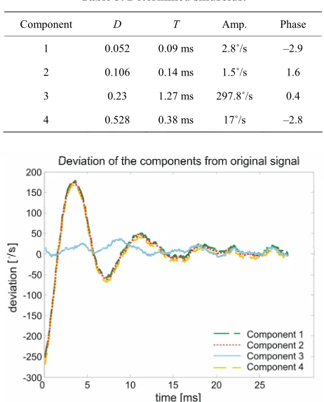
Table 3 shows the parameters of all determined damped
sine components for the step response of setting 2. Small amplitudes and time constants, as for component one, two and four, were used to differentiate irrelevant sinusoids, since the model order was four in the calculation. The characteristic sinusoid is component three.
Another possible criterion is the deviation from the original signal, shown in Figure 6. The error of compo-
nent 3 is the smallest through the whole time, especially in the relevant first time interval.
5. Summary
The approach described in this paper utilizes the Prony Analysis for assessing the velocity controller of electrical servo drives. Some known disadvantages of this analysis
Table 2. Results of Prony analysis for three velocity con- troller settings after different excitations.
Step Response Impulse Response
D T D T
Setting 1 0.64 2.6 ms 0.61 1.8 ms
Setting 2 0.28 1.3 ms 0.22 1.2 ms
Setting 3 0.56 1.5 ms 0.6 1.46 ms
Table 3. Determined sinusoids.
Component D T Amp. Phase
1 0.052 0.09 ms 2.8˚/s –2.9
2 0.106 0.14 ms 1.5˚/s 1.6
3 0.23 1.27 ms 297.8˚/s 0.4
4 0.528 0.38 ms 17˚/s –2.8
[image:5.595.63.280.520.696.2]were mitigated by confining the analysis to a time period after an excitation of the closed control loop. As result, different controller settings were distinguished and cor-rectly rated. Through some alteration of the algorithm, implementation in an industrial motion controller was enabled.
6. References
[1] R. Neugebauer, R. Schönherr, J. Quellmalz and H. Sch- legel, “Überwachung und Bewertung von Antriebsre- gelungen bei Verzicht auf zusätzliche Sensorik,” Proceed- ings of VDI-Congress Automation 2010, Baden-Baden, 15-16 June 2010, pp. 117-120.
[2] L. Desborough and T. Harris, “Performance Assessment Measures for Univariate Feedback Control,” The
Cana-dian Journal of Chemical Engineering, Vol. 70, No. 6, 1992, pp. 1186-1197. doi:10.1002/cjce.5450700620
[3] H. Gross, J. Hamann and G. Wiegärtner, “Elektrische Vorschubantriebe in der Automatisierungstechnik,” Publi- cis Corporate Publishing, Erlangen, 2006.
[4] H. Lutz and W. Wendt, “Taschenbuch der Regelung- stechnik: Mit Matlab und Simulink,” Harri Deutsch Verlag, Frankfurt, 2007.
[5] S. L. Marple Jr., “A Tutorial Overview of Modern Spec-tral Estimation,” Proceedings of the International Con-ference on Acoustics, Speech, and Signal Processing, Glasgow, 23-26 May 1989, pp. 2152-2157.
doi:10.1109/ICASSP.1989.266889