Frequency Control of Power System with Solar and Wind Power Stations by Using Frequency Band Control and Deadband Control of HVDC Interconnection Line

DOI: 10.4236/jpee.2018.69007 Sep. 25, 2018 48 Journal of Power and Energy Engineering

Frequency Control of Power System with Solar

and Wind Power Stations by Using Frequency

Band Control and Deadband Control of HVDC

Interconnection Line

Kimiko Tada

_{, Takamasa Sato}

_{, Atsushi Umemura}

_{, Rion Takahashi}

_{, Junji Tamura}

_,

Yoshiharu Matsumura

, Tsukasa Taguchi

, Akira Yamada

1_{Department of Electrical and Electronic Engineering, Kitami Institute of Technology (KIT), Kitami, Japan} 2_{Hokkaido Electric Power Co., Inc., Sapporo, Japan}

Abstract

In recent years, environmental problems are becoming serious and renewable energy has attracted attention as their solutions. However, the electricity gen-eration using the renewable energy has a demerit that the output becomes unstable because of intermittent characteristics, such as variations of wind speed or solar radiation intensity. Frequency fluctuations due to the installa-tion of large scale wind farm (WF) and photovoltaics (PV) into the power system is a major concern. In order to solve the problem, this paper proposes two control methods using High Voltage Direct Current (HVDC) intercon-nection line to suppress the frequency fluctuations due to large scale of WF and PV. Comparative analysis between these two control methods is pre-sented in this paper. One proposed method is a frequency control using a notch filter, and the other is using a deadband. Validity of the proposed me-thods is verified through simulation analyses, which is performed on a mul-ti-machine power system model.

Keywords

High Voltage Direct Current (HVDC), System Frequency Control, PV Power Generation, Wind Power Generation, Notch Filter, Deadband

1. Introduction

Recently, global warming and depletion of fossil fuels have been becoming se-rious all over the world, and in Japan nuclear power plants have been stopped

How to cite this paper: Tada, K., Sato, T., Umemura, A., Takahashi, R., Tamura, J., Matsumura, Y., Taguchi, T. and Yamada, A. (2018) Frequency Control of Power System with Solar and Wind Power Stations by Using Frequency Band Control and Dead-band Control of HVDC Interconnection Line. Journal of Power and Energy Engi-neering, 6, 48-63.

https://doi.org/10.4236/jpee.2018.69007

Received: August 22, 2018 Accepted: September 22, 2018 Published: September 25, 2018

Copyright © 2018 by authors and Scientific Research Publishing Inc. This work is licensed under the Creative Commons Attribution International License (CC BY 4.0).

http://creativecommons.org/licenses/by/4.0/

DOI: 10.4236/jpee.2018.69007 50 Journal of Power and Energy Engineering which the control performance is not sufficient. Therefore, by determining the frequency band in which the frequency adjustment ability decreases in the power system with renewable power sources installed, a notch filter capable of effec-tively extracting only this band can be designed. Then, using the designed notch filter, fluctuating power in that frequency band, which cannot be suppressed suf-ficiently in the power system with renewable power sources, is transmitted to another power system through the HVDC interconnection line. As a result, fre-quency fluctuations in the power system with renewable power sources are sup-pressed.

The other method is a frequency control using deadband. This control is very simple. Only when the frequency deviation in the power system with renewable power sources exceeds a threshold value, the frequency control of HVDC inter-connection line activates and the fluctuating power is transmitted to another system. In the case of the frequency control using notch filter, the frequency control of HVDC transmission line is always in operation. However in the case of the frequency control using deadband, the frequency control of HVDC transmission line is in operation only when the frequency deviation exceeds the threshold value. Therefore fluctuations in the HVDC transmission line power in the latter case become smaller than those in the former case.

The effectiveness of the above two proposed methods is verified by simulation analysis executed on PSCAD/EMTDC software (4.2.1).

2. Model System

2.1. Power System Model

The power system model used in this study and its parameters are shown in Figure 1. It is a modified version of the IEEE standard model with 9 buses [10] which is composed of 3 synchronous generators (SG1, SG2, and SG3). SG1 and SG2 are thermal power plants (SG1: 300 MVA, SG2: 200 MVA), and SG3 is a hydraulic power plant (100 MVA). Moreover, a WF (40 MVA), a PV station (60 MVA), HVDC interconnection line (60MVA), and three loads (Loads A, B, and C) are connected to the main system [11]. Their conditions are shown in Table 1. The HVDC transmission line is connecting the main modified 9-bus power system (System A) and another large power system (infinite bus, System B) and the positive direction of its power flow is from System A to System B.

2.2. Governor Model

DOI: 10.4236/jpee.2018.69007 51 Journal of Power and Energy Engineering Figure 1. Model system.

Table 1. Conditions of each generator.

Generator Rated MVA Frequency Control

SG1 Thermal 300 MVA LFC*1

SG2 Thermal 200 MVA GF*2

SG3 Hydro 100 MVA GF*2

SCIG*3 _{Wind Farm 40 MVA}

PV Solar 60 MVA

Total Load 480 MW

*1_{LFC: Load Frequency Control, *}2_{GF: Governor Free, *}3_{SCIG: Squirrel Cage Induction Generator.}

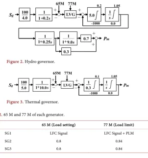
governor system. There are various frequency components in the power sup-plied to the power system from the wind generators and PV stations, resulting in frequency fluctuations of the power system. Conventional thermal and hydro governors control their turbine output to suppress the frequency fluctuations, in which short period components of from a few tens of seconds to a few minutes are controlled by the governor free (GF) operation and relatively long period components of from a few minutes to several tens of minutes are controlled by the load frequency control (LFC). These control blocks used in this paper are shown in Figure 2 and Figure 3 [12]. A hydraulic generator speed governor model used in the simulation analyses is shown in Figure 2, where

Sg: Rotation speed deviation

65M: Load setting (Output reference value) 77M: Load limit (65M + rated output × PLM [%])

PLM: Governor operating margin [%] (A percentage of the rated output) Pm: Turbine output

DOI: 10.4236/jpee.2018.69007 52 Journal of Power and Energy Engineering Figure 2. Hydro governor.

Figure 3. Thermal governor.

Table 2. 65 M and 77 M of each generator.

65 M (Load setting) 77 M (Load limit)

SG1 LFC Signal LFC Signal + PLM

SG2 0.8 0.84

SG3 0.8 0.84

shown in Figure 3 and Figure 4. Load frequency control (LFC) supplies output command signal to the power plants according to the frequency deviation. The LFC signal is input to 65M, and then, the output of each power plant is changed. The frequency deviation is input to the Low Pass Filter (LPF) to remove com-ponents of short period as shown in Figure 4, and then LFC signal is generated through PI controller. This is because the LFC is used to control frequency fluc-tuations with a long period of time. The angular frequency ωc (=2πf) of LPF is

set to 0.005 [Hz]. The governor models used in this paper are based on the stan-dard models of the Institute of Electrical Engineers of Japan.

2.3. Wind Turbine Model

Wind turbine model used in this paper is shown in Equations (1)-(5) [13].

( )

(

)

wtb p w

P = ρC λ β R V (1)

(

) ( )

(

)

p

C λ β _{= Γ −} β ₋ − Γ ₍₂₎

(

)

λ= ω (3)

(

)(

)

( )

( )

Γ = = (4)

( )

( )

M Ct R Vw

τ = ρ λ (5)

where, Pwtb: wind turbine output [W], λ: tip speed ratio, R: wind turbine radius

DOI: 10.4236/jpee.2018.69007 53 Journal of Power and Energy Engineering Figure 4. LFC system.

speed [m/s], ρ: air density [kg/m3_{], C}

p: power coefficient, Ct: torque coefficient,

τM: wind turbine torque [Nm].

2.4. PV System

PV model used in this study is shown in Figure 5 [8]. In this study, the PV model is expressed by a simple model using current sources, in which kilowatts data, PPV [kW], is used. Therefore, PV current (IPV) is calculated from PPV [kW]

and VPV [kV], and the obtained current (IPV) is entered to the grid from the

cur-rent sources. PV voltage (VPV) is fixed at 6.6 kV.

2.5. HVDC System

The HVDC system model used in this study is shown in Figure 6 [7] [9]. In this study, to shorten the calculation time of the simulation, the HVDC model is ex-pressed by the simple model [11] using controlled voltage sources instead of IGBT based inverter and rectifier.

2.5.1. Control Model of System Aa Side Converter

The control block of the converter that converts from three-phase AC to DC voltage is designed as shown in Figure 7. First, the phase angle is obtained by detecting the phase voltage Vr from the three-phase terminal voltage at the

con-verter. Next, the d-axis and q-axis components (Ird, Irq) of the current are

ob-tained from the phase angle and the three-phase current. Active power Pr and

reactive power Qr of the converter are controlled independently by the d-axis

and the q-axis components. For this purpose, the d-axis and q-axis components

(

)

ref-erence value Pref is determined so as to suppress system frequency fluctuations

(described later). Finally, the d-axis and q-axis voltages are converted to three-phase AC voltages. The parameters of PI controllers (PI1, PI2) are shown in Table 3.

2.5.2. Control Model of System B Side Inverter

The control block of the inverter that converts the DC voltage to the three-phase AC is designed as shown in Figure 8. As shown in Figure 8, the phase angle is obtained by detecting the phase voltage Vq from the three-phase terminal voltage

at the inverter. Next, the d-axis and q-axis components (Iqd, Iqq) of the current

DOI: 10.4236/jpee.2018.69007 54 Journal of Power and Energy Engineering Figure 5. PV model.

Figure 6. VSC-HVDC simple model.

Figure 7. Converter control system.

of the HVDC line and reactive power output Qq of the inverter are controlled by

DOI: 10.4236/jpee.2018.69007 55 Journal of Power and Energy Engineering Figure 8. Inverter control system.

Table 3. Parameters of PI controller.

PI1 PI2 PI3 PI4

Proportional gain 0.1 0.1 1.0 0.1

Integral time constant 0.01 1.0 0.1 1.0

2.6. DC-Link Model

The DC-Link model is shown in Figure 9, in which the DC-link voltage is ex-pressed by Equation (6) [7] [9].

(

)

(

)

dVdc dt= 1V Cdc dc P Pr− q (6)

where, Vdc: DC Voltage, Cdc: Capacitance of smoothing capacitor in the DC link

(50,000 μF), Pr: Active power of the converter, Pq: Active power of the inverter.

Rated voltage of the HVDC line is 250 kV.

2.7. Proposed Methods for Frequency Control in HVDC

Transmission Line

2.7.1. Frequency Band Control Using Notch Filter

Firstly frequency characteristics of System A are analyzed in order to clarify the frequency band in which the synchronous generators and their frequency con-trol systems in System A cannot suppress frequency fluctuations sufficiently. In order to perform the frequency characteristic analysis, System A of Figure 1 is expressed by using the simple frequency block model shown in Figure 10 [14] [15]. Figure 11 shows the result of frequency characteristics of System A, in which X-axis denotes frequency of input power variation and Y-axis denotes the maximum frequency deviation in System A. “No frequency control” in Figure 11 shows the result calculated from transfer function from output variations of WF and PV to frequency variations of System A, which is obtained from the frequency block model.

DOI: 10.4236/jpee.2018.69007 56 Journal of Power and Energy Engineering Figure 9. DC-Link control block.

Figure 10. Simple frequency block model.

Figure 11. Frequency characteristics of System A.

A cannot suppress sufficiently. Since the permissible range of power system fre-quency deviation in Japan is, in general, within ± 0.2 Hz, the filter is designed so that the maximum frequency deviation is equivalent to 0.2 Hz. “with Notch fil-ter” in Figure 11 are the results. In this paper, the transfer functions of the de-signed notch filter is shown in Equation (7), where ζ1 is damping coefficient, ωc1

is center angular frequency, and their values are set to ζ1= 4.9, ωc1 = 0.387

re-spectively.

( )

(

) (

)

1 2 1 1 1

c c c

notch

H s = s +ω s + ζ ω s+ω ₍₇₎

Figure 12 shows a block diagram to determine reference output of HVDC transmission line, where Δf is the frequency deviation in System A and Pref is the

reference for HVDC line power. In the case of the proposed method, by passing Δf through the notch filter and subtracting the filter output from Δf, the fluctu-ating frequency components that cannot be suppressed sufficiently is obtained, and finally, by adding the steady state reference value for HVDC line power, PDC0

(=0.5 [p.u.] in this study), to it, Prefis determined. Pref is limited within PDC0± 0.1

DOI: 10.4236/jpee.2018.69007 57 Journal of Power and Energy Engineering Figure 12. Block diagram to determine HVDC line output using notch filter.

fluctuations of HVDC line power. P gain in Figure 12 is set to %KG = 15.0,

which is the system constant of System A. The equation about the system con-stant %KG is shown in Equation (8). KG is the amount of total generator output

which needs to change the system frequency by 1 [Hz].

(

)

%K_G = K_G×100 sum of the Rated Capacities of Parallel Generator ₍₈₎

2.7.2. Frequency Control Using Deadband

Figure 13 shows a block diagram of the proposed frequency control with dead-band [16] [17] for the HVDC line, where Pref denotes a reference for HVDC line

power flow and it is determined according to the frequency deviation ∆f [Hz] of the main system (System A). In Figure 13, ∆P = 0 when ∆f [Hz] is less than the threshold value “a” [Hz] in the deadband, and ∆f * P gain is sent to the adder when ∆f [Hz] is greater than the threshold value. Target value Pref of the HVDC

line flow is calculated by adding ∆P to the steady state reference value, PDC0 (=

0.5 [p.u.] in this study). Prefis limited within PDC0± 0.1 [p.u.] by using the hard

limiter as shown in Figure 13 also in this case. Therefore, HVDC line flow is composed of compensating component for the frequency fluctuations and the steady state reference. In Figure 14, the output image of the deadband is shown. The threshold value “a” of the deadband is set to 0.05 [Hz] in this paper, and P gain is set to %KG= 15.0, which is the system constant of System A. The

equa-tion about the system constant %KG is shown in Equation (8).

3. Simulation Results

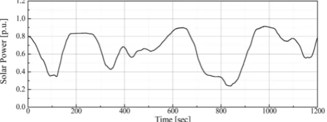
To confirm the effectiveness of the proposed methods, simulation analyses for the model system of Figure 1 are performed on PSCAD/EMTDC software for the three cases; Case 1: No frequency control, Case 2: Frequency control with Notch filter in Figure 12, Case 3: Frequency control with Deadband shown in Figure 13. These 3 cases are shown in Table 4. The wind speed data shown in Figure 15 is input into the wind turbine model in the simulation analyses. This is real wind speed data measured in Hokkaido Island, Japan. The calculated output of wind turbine generator is shown in Figure 16. The PV output data shown in Figure 17 is used in the simulation analyses. This is also real PV data measured in Hokkaido Island, Japan. The total of this output of wind turbine generator and PV station is shown in Figure 18.

DOI: 10.4236/jpee.2018.69007 58 Journal of Power and Energy Engineering Figure 13. Block diagram to determine HVDC line output using deadband.

Figure 14. Output image in deadband.

Figure 15. Wind speed data.

Figure 16. Output of wind power generator.

DOI: 10.4236/jpee.2018.69007 59 Journal of Power and Energy Engineering Figure 17. Output of PV station.

Figure 18. Total output of WF and PV.

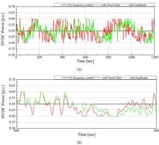
DOI: 10.4236/jpee.2018.69007 60 Journal of Power and Energy Engineering Figure 20. (a) Comparison of HVDC transmission power. (b) Comparison of HVDC transmission power (enlarged).

Table 4. Study cases.

Case Description

1 _{(HVDC transmission power is set to 0.5 p.u.)} No frequency control

2 _{(HVDC transmission power is controlled within 0.5 ± 0.1 p.u.)} Frequency control with Notch filter

3 _{(HVDC transmission power is controlled within 0.5 ± 0.1 p.u.)} Frequency control with Deadband

Table 5. Maximum deviation and standard deviation of system frequency.

Case 1 (No Frequency

control )

Case 2 (Frequency control

with Notch filter)

Case 3 (Frequency control

with Deadband) Maximum Frequency

Deviation +∆f [Hz] 0.234 0.182 0.179

Maximum Frequency

Deviation −∆f [Hz] −0.225 −0.184 −0.172

Standard Deviation [Hz] 0.0805 0.0728 0.0704

DOI: 10.4236/jpee.2018.69007 61 Journal of Power and Energy Engineering Maximum Deviation

of HVDC power +∆Pref [p.u.]

0.0 0.100 0.100

Maximum Deviation of HVDC power

−∆Pref [p.u.]

0.0 −0.100 −0.100

Standard Deviation

of HVDC power [p.u.] 0.0 0.0561 0.0438

standard deviation of the HVDC line power, from which it is also seen that the HVDC power fluctuations can be suppressed effectively in Case 3.

4. Discussion

In the simulation analysis of Section 3, two proposed methods for stabilizing the frequency fluctuations of system A have been analyzed. From Table 5, it is seen that the frequency control using the deadband (Case 3) can suppress the fre-quency fluctuations slightly more than the frefre-quency control using the notch fil-ter (Case 2). This is because, the frequency control based on the notch filfil-ter suppresses the frequency fluctuations just within ±0.2 Hz while the control using deadband suppresses all components of the frequency fluctuations whenever the fluctuations become over the threshold value. On the other hand, it is seen from Table 6 that the standard deviation of the HVDC line power flow is less in the frequency control using the deadband (Case 3) than in the control using the notch filter (Case 2). This is because the HVDC line power in Case 2 always fluctuates while the HVDC line power in Case 3 does not so fluctuate as can be seen from Figure 20. HVDC line power control always activates in Case 2 but it activates in Case 3 only when the frequency fluctuations become over the thre-shold value. Therefore the HVDC line power flow fluctuations are less in Case 3 than Case 2. Considering these aspects, it is concluded that the frequency control using the deadband (Case 3) is superior to the frequency control using the notch filter (Case 2).

5. Conclusion

DOI: 10.4236/jpee.2018.69007 62 Journal of Power and Energy Engineering with large amount of wind power generation and solar power generation. The proposed method can contribute to a design of frequency control system of power system which includes large amount of wind power generation and solar power generation and is connected to other power system through a HVDC in-terconnection line. The authors are planning to include the balancing control of the HVDC line into the proposed method.

Acknowledgements

This study was supported by the Grant-in-Aid for Scientific Research (B) from The Ministry of Education, Science, Sports and Culture of Japan.

Conflicts of Interest

The authors declare no conflicts of interest regarding the publication of this pa-per.

References

[1] Global Wind Energy Council (GWEC). (2015) Annual Market Update 2015, Global Wind Report. http://gwec.net/

[2] Renewable Energy Policy Network for the 21st Century (REN21). Renewables 2017 Global Status Report.

http://www.ren21.net/status-of-renewables/global-status-report/

[3] Liu, H. and Chen, Z. (2015) Contribution of VSC-HVDC to Frequency Regulation of Power Systems with Offshore Wind Generation. IEEE Transactions on Energy Conversion, 30, 918-926. https://doi.org/10.1109/TEC.2015.2417130

[4] Guan, M., Cheng, J., Wang, C., Hao, Q., Pan, W., Zhang, J. and Zheng, X. (2017) The Frequency Regulation Scheme of Interconnected Grids with VSC-HVDC Links.

IEEE Transactions on Energy Conversion, 32, 864-872.

[5] Li, Y., Xu, Z., Østergaard, J. and Hill, D.J. (2017) Coordinated Control Strategy for Offshore Wind Farm Integration via VSC-HVDC for System Frequency Support.

IEEE Transactions on Energy Conversion, 32, 843-856.

https://doi.org/10.1109/TEC.2017.2663664

[6] Wang, L., Lin, C.-Y., Wu, H.-Y. and Prokhorov, A.V. (2017) Stability Analysis of a Microgrid System with a Hybrid Offshore Wind and Ocean Energy Farm Fed to a Power Grid Through an HVDC Link. IEEE Industry Applications Society, 54, 2012-2022. https://doi.org/10.1109/TIA.2017.2787126

[7] Jahan, E., Hazari, Md.R., Rosyadi, M., Umemura, A., Takahashi, R. and Tamura, J. (2017) Simplified Model of HVDC Transmission System Connecting Offshore Wind Farm to Onshore Grid. Proceedings of the IEEE PES PowerTech, Manchester, 18-22 June 2017, 1-6.

DOI: 10.4236/jpee.2018.69007 63 Journal of Power and Energy Engineering

[10] Anderson, P.M. and Found, A.A. (1944) Power System Control and Stability. IEEE Press, New York.

[11] Rosyadi, M., Umemura, A., Takahashi, R., Tamura, J., Uchiyama, N. and Ide, K. (2015) Simplified Model of Variable Speed Wind Turbine Generator for Dynamic Simulation Analysis. IEEJ Transactions on Power and Energy, 135, 538-549.

https://doi.org/10.1541/ieejpes.135.538

[12] Liu, J., Rosyadi, M., Umemura, A., Takahashi, R. and Tamura, J. (2014) A Control Method of Permanent Magnet Wind Generators in Grid Connected Wind Farm to Damp Load Frequency Oscillation. IEEJ Transactions on Power and Energy, 134, 393-398. https://doi.org/10.1541/ieejpes.134.393

[13] Wasynczuk, O., Man, D.T. and Sullivan, J.P. (1981) Dynamic Behavior of a Class of Wind Turbine Generators during Random Wind Fluctuations. IEEE Power Engi-neering Review, PER-1, 47-48. https://doi.org/10.1109/MPER.1981.5511593

[14] Koiwa, K., Tahara, S., Tamura, J. and Liu, K.-Z. (2016) A Study on the Design of Battery Capacity and Control System Based on the Frequency Characteristics of Power System. IEEJ Transactions on Power and Energy, 136, 719-727.

https://doi.org/10.1541/ieejpes.136.719

[15] Tahara, S., Koiwa, K., Umemura, A., Takahashi, R. and Tamura, J. (2015) Frequen-cy Characteristic Analysis of Power System and Its Application to Smoothing Con-trol of Wind Farm Output. Proceedings of the 10th International Conference on Ecological Vehicles and Renewable Energies (EVER), Monaco, 31 March-2 April 2015, 1-6.

[16] Ono, T. and Arai, J. (2012) Frequency Control with Dead Band Characteristic of Battery Energy Storage System for Power System Including Large Amount of Wind Power Generation. IEEJ Transactions on Power and Energy, 132, 709-717.

https://doi.org/10.1541/ieejpes.132.709

[17] Yoshida, Y., Koiwa, K., Umemura, A., Takahashi, R. and Tamura, J. (2015) Power System Frequency Control with Dead Band by Using Kinetic Energy of Variable Speed Wind Power Generator. Proceedings of the 2015 IEEE Energy Conversion Congress and Exposition (ECCE), Montreal, 20-24 September 2015, 470-476.