Random Search Algorithm for the Generalized Weber Problem

Random Search Algorithm for the Generalized Weber

Problem

Lev Kazakovtsev

Department of Information Technologies, Siberian State Aerospace University, Krasnoyarsk, Russian Federation. Email: [email protected]

Received 2012.

ABSTRACT

In this paper, we consider the planar multi-facility Weber problem with restricted zones and non-Euclidean distances, propose an algorithm based on the probability changing method (special kind of genetic algorithms) and prove its effi-ciency for approximate solving this problem by replacing the continuous coordinate values by discrete ones. Version of the algorithm for multiprocessor systems is proposed. Experimental results for a high-performance cluster are given.

Keywords: Discrete Optimization; Weber Problem; Random Search; Genetic Algorithms; Parallel Algorithm

1.

Introduction

Location problems are a special class of optimization problems [1]. A single-facility Weber problem is a prob-lem of searching for a point X that the sum of weighted distances from X to some existing points A1, A2... ,AN is

minimum [2].

( )

X = wL

(

X,A

)

min.

F i

N

= i

i →

∑

1

(1)

Here, wiis a weight of the i'th point, L(A,B) is the

distance between A=(a1,b1) and B=(b1,b2). In the

Euc-lidean metrics l2,

( ) (

) (

2 2

)

2.

2 1

1 b + a b

a = B A,

L − − (2)

But, other types of distances have been exploited. A review of exploited metrics is presented in [3]. Distance functions based on altered norms are investigated in [4, 5]. Problems with weighted one-infinity norms are solved in [6]. Asymptotic distances [7] and weighted sums of order p [8] are also.

Also, the rectangle [4] (or Manhattan) metrics l1 is

well investigated. Here,

( ) |

A,B = a1 b1

| |

+a2 b2

|

.

L − − (3)

Manhattan metric can be used for fast approximate solution instead of Euclidean metric.

Weber (or Fermat-Weber) problem is a generali-zation of a simple Fermat problem and has series of ge-neralized formulations.

Multi-facility problem (Multi-Weber problem) is a generalization of the single-facility problem [9]:

(

X ,X

)

= wL

(

X ,A

)

min.

F _{j i}

N = i

M = j

i

M

∑∑

→

1 1

1,... (4)

The problem is searching for M additional places for new facilities Xj,1≤ j≤M.

Or, in other case [9], the objective function is de-fined as (minsum problem):

(

X ,X

)

= w L

(

X ,A

)

min.

F min _{j i}

M j j, N

= i

i

M

∑

_{1≤ ≤} →

1

1,,... (5)

Also, the problem can include the restricted areas, barriers etc. In case of restricted zones, the optimization problem, in general, includes constraints:

Z j R

X ∉ (6)

where RZ is a set of restricted coordinates.

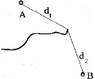
[image:1.595.343.507.569.705.2]

In case of barriers, the distance between 2 points is, in general, non-Euclidean (Fig.1)

Here, the distance between points A and B is the sum of distances d1 and d2 (piano movers distance [10]).

Continuous (regional) Weber problem deals with finding a median for a continuum of demand points. In particular, we consider versions of the ''continuous k-median (Fermat-Weber) problem'' where the goal is to select one or more center points that minimize the weighted distance to a set of points in a demand region [11]. If the existing facilities are distributed in some compact area Ω∈Rn then the single-facility continuous Weber problem [12] is to find X so that

( )

X = w L

(

X,A

) ( )

dμA min.

F _{i i}

Ω N

= i

i

∫

→

∑

1

(7)

where μ

( )

A_i is the expectation of the fact that the i'th customer is placed in some area. If this expectation is equal among some area, i.e., if i'th customer is uniformly (equably) distributed in the area Ω_i then

( )

( ) ( )

,

1

min dA A A X, L w = X

F i

i Ω N

= i

i

∫

→

∑

ρ (8)

( )

  

∉ ∈

i i i

Ω

A

Ω

A = A

, 0

, 1

ρ . (9)

In case of continuous (regional) multi-Weber prob-lem,

(

)

(

X ,A

)

( )

AdA min. L

w =

= X , , X F

i j i

Ω n i m

M j j, N

= i

i M

→

∫

∑

_{≤ ≤} ρ

1 1 1...

(10)

In this paper, we propose an algorithm for approx-imate solving the problem (10) with constraints (6) where the distance function L() is an arbitrary monotone function. In the example given this function is the well known path loss function implemented to calculate the radio-propagation features of the area (media).

2.

Related Works, Existing Methods

The Weber problem locates medians (facilities) at continuous set of locations in the Euclidean plane (or plane with an arbitrary metrics in generalized case). Ha-kimi proposed similar problem statement for finding me-dians on a network or graph [13, 14], proved that an op-timal absolute median is always located at a vertex of the graph, thus providing a discrete representation of a con-tinuous problem and generalized the absolute median to find p medians. Solutions consisting of p vertices are called p-medians of the graph.

In the case of discrete coordinates, considering all cells of discrete rectangular coordinate system as feasible points, we have p-median problem. But the dimension of such problem is very large if the discretization is precise enough. In general, p-median problem is NP-hard, the

polynomial time algorithm is available on trees only [15] In [16], authors utilized a network flow procedure (an algorithm for p-median problem) to solve the mul-ti-facility location problem with rectilinear distances . In case of the Weber problem (except one with Manhattan or similar metric) [17], the sum of the edges weights is not equal to distance in the problem with the discrete coordinate grid.

Drezner and Wesolowsky [18] researched the con-tinuous problem under an arbitrary lp distance metric.;

and, in [6], authors formulated the well-known “block-norm” for the distances involved.

The unconstrained problem with the mixed coordi-nates (discrete and continuous) is considered in [17].

For generalized multi-Weber problem with re-stricted zones and barriers, only some special cases are considered. Bischoff et al. [18] provided two heuristics for the multi-Weber problem with barriers, and reported that their algorithms can attain solutions of reasonably sized multifacility location problems with barriers, both with regard to computation time and solution quality.

Having transformed our continuous Weber problem into problem with discrete coordinate grid, we have a combinatorial discrete optimization problem.

Most exact solution approaches to the problem of discrete (combinatorial) optimization are based on branch-and-bound method (tree search) [19, 20, 21], most them are in the complexity class NP-hard and re-quire searching a tree of the exponential size and even parallelized versions of such algorithms do not allow us to solve some large-scale pseudo-Boolean optimization problems in acceptable time.

The heuristic random search methods do not guar-antee any exact solution but they statistically optimal. I.e. the percent of the problems solved “almost optimal” grows with the increase of the problem dimension [19].

Being initially designed to solve the unconstrained pseudo-Boolean optimization problems, the probability changing method (MIVER) is a random search method organized by the following common scheme [19, 20, 22]. Algorithm 1

1. k=0, the starting values of the probabilities Pk={pk1,

pk2, ... , pkN} are assigned where pkj=P{xj=1}. Correct

setting of the the starting probabilities is a very signifi-cant question for the constrained optimization problems.

.

2. With probability distributions defined by the vector Pk, we generate a set of the random Boolean vectors Xk.

3. The function values are calculated: F(Xki).

4. Some function values from the set F(Xk) and

cor-responding points Xki are picked out (for example, point

with maximum and minimum values).

5. On the basis of results in item 4, vector Pk is

mod-ified.

7.Otherwise, stop.

The modified version of the variant probability method, offered in [22, 23] allows us to solve problems with dimensions up to millions of Boolean variables.

3.

Discrete Problem Statement

Let's consider the problem (10) with constraints (6) in case when the coordinate grid is discrete. For most prac-tically important problems, the solution of such approx-imated (discretized) problem is enough. Moreover, the distance measurement is always finite.

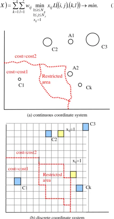
The transformation of the continuous coordinates into discrete coordinate grid is shown in Figure 2. The area is divided into Nx columns and Ny rows and the whole area

forms a set of cells. In this case, the integral in formula (10) of the regional Weber problem is transformed back into a sum (5) of a Multi-Weber problem. The problem is to select p cells where the new facilities will be placed so that

( )

X = w x L

(

( ) ( )

i,j ,k,l

)

min.

F ij

= x

N j x

N i x

N

= k

y N

= l

ij

ij y

→

≤ ≤≤ ≤

∑∑

1 1 1 1 1

1 min (11)

C1

C2 C3

Ck

cost=cost1 cost=cost2

Restricted area

A1

A2

(a) continuous coordinate system

C1

C2

C3

Ck cost=cost1

cost=cost2

Restricted area

xij=1

xij=1

[image:3.595.71.272.318.702.2]

(b) discrete coordinate system

Figure 2. Problem Transformation

     

 

     

 

NxNy Nx

Nx

Ny Ny

x x

x

x x

x

x x

x = X

... ... ... ... ...

... ...

2 1

2 22

21

1 12

11

(12)

with constraints

( )

F. x

N

= i

y N

= j

ij

z ij

N

x

;

R

j

i,

=

x

≤

∈

∀

∑∑

1 1

0

(13)

Here, X is a matrix of Boolean variables, Rz is a set

of cells restricted for facility placement, L() is a distance function, in general, arbitrary but monotone. If we have a problem with barriers, this function is calculated as shown in Fig.1. wij is the weight of the cell (i,j), NF is

quantity of facilities to be placed.

Also, the problem may have additional constraints. As an example of the problem (11-13), we will consider a problem of antennas placement.

Here, we have a map with discrete coordinates, each cell has its weight which is a measurement of its importance to be covered with stable RF signal from any of antennas. The cells can contain different kinds of ob-stacles (walls, trees etc). As the distance function, we can use the well-known path loss function [24] calculated as

( )( )

(

i,j k,l

)

=20log

( ) ( )

i,j ,k,l +L

(

( ) ( )

i,j,k,l

)

.

L OBST (14)

Here, LOBST is the obstacle path loss which is

calcu-lated algorithmically as loss at all the obstacles (depend-ing on their material and thickness) along the path be-tween the cells (i,j) and (k,l). The RF absorbing proper-ties of the environment elements are available from the information tables [25]. In our distance function, we do not take into consideration the antenna gain since this parameter does not depend on antennas placement.

In continuous coordinates, the objective function is monotone. We have a pseudo-Boolean optimization problem (11-14). The total quantity of variables of our problem is NxxNy. Thus, even in case of 100x100

coor-dinate grid, we have a problem with 10000 variables. Since the objective function is given algorithmical-ly, the distribution of the computational tasks between the parallel processors or cluster nodes is important.

In this paper, we do not consider greedy search al-gorithms [26]) though they can be used to improve the results of the random search methods.

4.

Serial and Parallel Realization

have matrix of Boolean variables X instead of a vector. It does not change the general scheme of our algorithm but simplifies the further description.

At the step of initialization (Step 1 of the Algorithm 1), all the variables p (components of the probability

matrix P) are set to their initial values (0<pi<1 ∀

P

p

i

∈

). Then (Step 2), we generate the matrices X of

optimized boolean variables. In our case of constrained problem, the large values of matrix P components gener-ate the values of X which are out of the feasible solutions area due to the constraints (13). Due to the constraints (13), the optimal initial values of the matrix P compo-nents do not exceed NF/(Nx Ny) [30].

Instead of maximum number of steps R (Step 6), we can use the maximum run time as the stop condition. In some cases, it is reasonable to use the maximum number of steps which do not improve the result achieved.

In the cycle (i=1,N), we generate the set of N ma-trices Xki in accordance with the probability matrix P.

Then, the objective function is calculated for each Xki.

To take into consideration the constraints (13), we modify the step of X exemplars generation.

Algorithm 2

∑

=

Y

N j ij

i

=

p

S

1 .

1. XSET =Ø; n=0;

2. while n<NF do

2.1. for each i in (1,Nx): ;

2.2. rx=Random();

2.3.

S

_x

=

r

_x

∑

_iN₌Y

S

_i 1 ;

2.4. select minimum i so that

∑

i_k=1

S

_i

≥

S

_x ;

2.5. ry=Random();

2.6.

S

_y

=

r

_y

S

_i :

2.7. select minimum j so that

∑

_lj₌₁

p

_il

≥

S

_y ;

2.8. if

(

i

,

j

)

∈

R

_Z then goto 2.2

2.9. else,

X

SET

=

X

SET

∪

( )

i,

j

; n=n+1; goto 2; Here, XSET is a set of coordinates (numbers of

col-umns and rows) of the resulting matrix X which are equal to 1, NF is quantity of the facilities placed, Random() is a

function with random value in range [0, 1).

The solution of different practical problems [22] shows the best result if we use the multiplicative adapta-tion of elements of matrix P with rollback procedure [27]. In this case, the components of the matrix P are never set to the value of 0 or 1 which may cause that all the further generations of the X matrix very similar.

In Algorithm1, all Boolean variables are considered as independent and the value of an element pij of the

ma-trix P at the k'th step can be calculated as

( ) ( ) ( )

∑∑

∑∑

− − −

⋅

⋅

Nx

= l y N = m j i, , k j i, k, x N = l y N = m j i, , k j i, k, j i, , k j i, k,

p

d

p

d

p

p

1 1 1 1 1 1 1

=

. (15)

Here, dk,i,j is the adaptation coefficient,

max k j, i,

x

and min k j, i,

x

are the exemplars of the matrix X giving the max-imum and the minmax-imum values of the objective function (11). In case of multiplicative adaptation, dk,i,j does not

depend on the step number k. In this case, the absolute value of adaptation step depends on the corresponding value of pkj.

In case of Weber problem, we consider the va-riables xij as dependent from each other. As follows from

the common sense (and proved experimentally), if the objective function has maximum value with Xworst so that

1

=

x

i,minj,k then, with some probability, the results at the

next steps will be better if

x

i,minj,k

=

1

or in some

sur-rounding area: S S S S k j , i

N

+

j

j

N

j

,

+N

i

i

N

i

x

* * * max , * *

*

1,

≤

≤

−

≤

≤

−

=

(16)

where NS is the width and height of the surrounding area.

The value of the coefficient d must be bigger for the points close to (i,j) for farther points, it must tend to 0.

We used the following formulas: w

*

/ k,i,j j i, k, j i,

k, =d d

d

;

(17)

( )

( )

(

)

(

)

       ± ∉ ∨ ∨ ± ∉ ± ∈ ∧ ± ∈ ] [ ] [ , 1 ] [ ^ ] [ , 1 / 1 * * * * * * * 0 * S S j i, k, S S j i, k, N j j N j i = d N j j N j i j i, , j , i L + d + = d (18)

(

)

( )

(

)

(

)

       ± ∉ ∨ ∨ ± ∉ ± ∈ ∧ ∧ ± ∈ ] [ ] [ 1, ] [ ] [ , 1 / 1 w w w 0 S w S w j i, k, S w S w w j i, k, N j j N j i = d N j j N j i j i, , j , i L + d + = d . (19)

Here, (i*,j*) and (iw,jw) are the closest points so that 1 min , * * = x k j ,

i and xw w, =1

worst k j ,

i correspondingly, X

worst _is

an exemplar of the X matrix with minimum objective function among the generated set.

lo-cal minimum. The rollback procedure helps to avoid that situation. It resets the values of P. The rollback is per-formed after several steps which do not improve the best objective function value.

The best results are demonstrated with methods of partial rollback procedure which change some part of P matrix components or change all the components so that their new values depend on previous results. We can use the following rollback formula:

pkij = (pk-1 i j +qk p0 )/(1+qk), if pk-1 i j <p0. (20)

Here, p0 is the initial value of the probability, we

assume that it is equal to the average value of the ele-ments of the matrix P. The coefficient qk may be constant

or vary depending on the results of previous steps. For example, it may depend on the quantity of the steps which do not improve the minimum result (sm).

qk = w / sm. (21)

The coefficient w must be chosen experimentally. The adaptation of our algorithm for multiprocessor systems with shared memory can be performed by the parallel generation of the exemplars of the X matrix and their estimation. If our system has NP processors,

the cycle of generation of N exemplars of the matrix X can be divided between the processors. Each processor has to generate N/Np exemplars of the matrix X and cal-culate the value of the objective function, left parts of the constraint conditions and calculate the modified objec-tive function values. Realization of such parallelization with OpenMP library with the appropriate compiler is very simple, actually, in Fortran or C, only a line with “parallel do” pragma before the cycle realizing the Step 2 of Algorithm1 is needed.

Organizing of the parallel thread takes significant computational expenses. In [27], authors estimate that expenses as 1000 operations of real number division. The experiments [23] at 4-processor system with linear 100-dimension problem show that the parallel version runs 2.8 times faster than the serial one. For large-scale problems with millions of variables, the parallel effi-ciency is almost ideal (0.95-0.97 for 1000 variables).

5.

Numerical Results

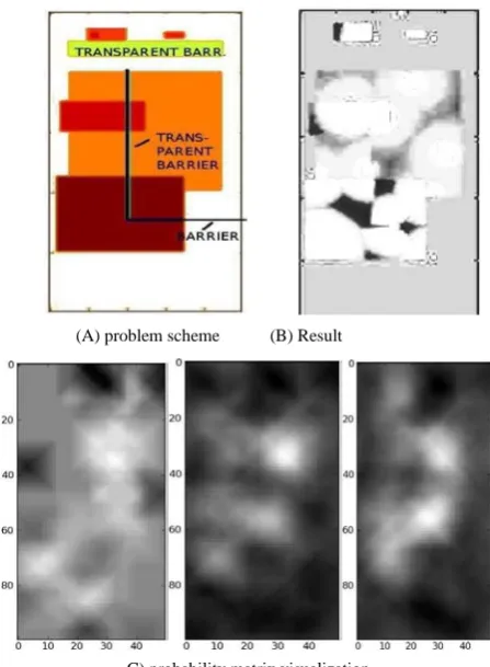
For testing purposes, we used a planar problem (11-14) with Nx=200, Ny=400. The map of our problem is shown

in Fig.4, part A. Dark areas correspond to the cells with the higher weight (important points), white with zero weight (points where RF-coverage is not important). The scheme has 3 obstacles (barriers).

Since our algorithm with the rollback procedure is a special case of the multistart algorithm, parallel multis-tart performed by different nodes of a cluster is allowed. In case of the problem (14), a cluster of 8 independent nodes (no message passing) achieve the same result as a single node spending approximately twice faster (47% - 59% of single node time). So, parallel efficiency

coeffi-cient is 0.21-0.27 for such cluster. The experiments were performed in the Argo cluster [28] (ICTP, Trieste, Italy).

For the parallel version for multiprocesor systems with OpenMP, the parallel efficiency coefficient is 0.92-0.95 for the problems of dimension 100x100 and grows with the dimension of the problem. For our testing example, the paralel efficiency is 0.94-0.95. The average efficiency is calculated after 10 runs for 5 different test-ing problems with different schemes similar to that shown in Fig.3, part A.

The parallel efficiency was calculated with the fol-lowing scheme. First, the serial version of the algorithm was implemented. The stop condition was its running for 5 min. The objective function value achieved was fixed as F*.Then the parallel version ran for the same problem with the stop condition F(X)≥F*.

The comparison of the efficiency of the algorithm with the existing methods is subject of the further re-search.

The algorithm is an anytime-algorithm. The deci-sion maker can stop the process of solving if the results seem to be appropriate. The results can be easily visua-lized (Fig.4, part B). Here, the dark areas are the areas with inappropriate signal level (customer regions situated too far from the facilities placed). The probability matrix can also be easily visualized (Fig.3, part C) and show the regions of most intensive search.

(A) problem scheme (B) Result

[image:5.595.310.534.396.701.2]

C) probability matrix visualization

6.

Conclusion

Modified random search algorithm based on probability changing method can be used for approximate solving planar generalized multi-Weber problem with non- Euc-lidean monotone distance function. Modern computing facilities (multiprocessor systems, low-cost clusters) al-low solving problems with appropriate precision. In the case of the MPI cluster for random search problems, ex-pensive high-performance network is not needed because of absence of any data traffic.

REFERENCES

[1] G. Wesolowsky, ''The Weber Problem: History and Perspectives'', Location Science, 1,1993, pp. 5–23. [2] R.Chen, ''Location Problems with Costs Being Sums

of Powers of Euclidean Distances'', Computers & Ops. Res., 11, 1984, pp.285–294

[3] Z. Drezner and H. Hawacher, ''Facility Location: Applications and Theory'', Berlin,, Springer-Verlag, 2004.

[4] R.F. Love and J.G. Morris, ''Computation Procedure for the Exact Solution of Location-Allocation Prob-lems with Rectangular Distances'', Naval Research Logistics Quarterly, 22, 1975, pp.441–453. doi: 10.1002/nav.3800220304

[6] J.E. Ward and R.E. Wenll, ''Using Block Norms for Location Modeling'', Operations Research, 33, 1985, pp.1074–1090. doi: 10.1287/opre.33.5.1074

[5] R.F.Love, W.G.

[12] M. Gugat and B. Pfeiffer, ''Weber Problems with Mixed Distances and Regional Demand'', Math Meth Oper Res, issue 66, 2007, pp.419–449.

doi:10.1007/s00186-007-0165-x

[13] S.L. Hakimi, ''Optimum Locations of Switching Centers and the Absolute Centers and Medians of a Graph'', Operations Research, 12(3), 1964, pp.450–459. doi: 10.1287/opre.12.3.450

[14] S.L. Hakimi, ''Optimum Distribution of Switching Centers in a Communication Network and Some lated Graph Theoretic Problems'', Operations Re-search, 13(3), 1965, pp.462–475. doi: 10.1287/opre.13.3.462

[15] O. Kariv and S.L. Hakimi, ''An algorithmic ap-proach to network location problems. II. The p-medians'', SIAM Journal on Applied Mathematics, 37(3), 1979, pp.539–560. oi: 10.1137/0137041 [16] A.V. Cabot, R.L. Francis and M.A. Stary, ''A

Net-work Flow Solution to a Rectilinear Distance Facility Location Problem'', American Institute of Industrial Engineers Transactions 2, 1970, pp. 132–141. [17] S. Stanimirovic, M. Ciric, ''Single-facility Weber

Location Problem Based On The Lift Metric''. http://arxiv.org/abs/1105.0757

[18] M. Bischoff, T. Fleischmann and K. Klamroth, ''The Multi-Facility Location-Allocation Problem with Polyhedral Barriers'', Computers and Operations Re-search, 36, 2009, pp.1376–1392. doi: 10.1016/j.cor.2008.02.014

[19] A.N. Antamoshkin, ''Optimizatsiya Funktsionalov s Bulevymi Peremennymi'' (''Optimization of Func-tionals with Boolean Variables''), TGU, Tomsk, 1987 [20] A.Antamoshkin, H.P. Schwefel, A. Toern, G. Yin

and A.Zhilinskas, ''System Analysis, Desing and Op-timization. An Introduction'', Ofset, Krasnoyarsk, 1993

[21] Yu. Finkelstein et al. ''Diskretnaya Optimzatsiya'' (''Discrete Optimization''), Metody Optimizatsii v Ekonomiko-Matematicheskom Modelirovanii, Nauka, Moscow, 1991, pp. 350-367

[22] L.Kazakovtsev, “Adaptive Model of Static Routing for Traffic Balance between Multiple Telecommuni-cation channels to different ISPs”, http://citeseerx.ist.psu.edu/viewdoc/download?doi=1 0.1.1.102.9445&rep=rep1&type=pdf (accessed 01.08.2012)

[23] L.A.Kazakovtsev and A.A.Stupina, ''Parallelnaya Realizatsiya Metoda Izmenyayushikhsya Veroyatnostey'' (''Parallel Realization of the Proba-bility Changing Method''), Sovremennye problemy nauki i obrazovaniya, №4, 2012, http://www.science-education.ru/104-6810

[24] T.S. Rappaport, ''Wireless Communications: Prin-ciples and Practice'', 2nd ed.–IEEE Press, 2002 [25] J.Hu and E. Goodman, ''Wireless Access Point

Configuration by Genetic Programming'', in Evolu-tionary Computation, 2004. CEC2004. Congress on, vol.1, 2004,pp. 1178- 1184

Truscott and J. Walker, ''Terminal Location Problem: A Case Study Supporting the Status Quo'', J. Opl Res. Soc., 36,1985, pp.131-136. doi:10.1057/jors.1985.26

[7]. M.J. Hodgson, R.T. Wong and J.Honsaker, ''The P-Centroid Problem on an Inclined Plane'', Opera-tions Research, Issue 35,1987, pp. 221–233. doi: 10.1287/opre.35.2.221

[8] J. Brimberg and R.F.Love, ''Properties of Ordinary and Weighted Sums of Order p Used for Distance Estimation'', Recherche Operationnelle, Issue 29,1995, pp. 59–72.

[9] L. Cooper, ''An extension of the generalized Weber problem'', Journal of Regional Science, Vol.8, Issue

2, 1968, pp. 181–197l. doi:

10.1111/j.1467-9787.1968.tb01323.x

[10] M.M. Deza and E. Deza, ''Encyclopedia of Distances'', Springer Verlag, 2009. doi: 10.1007/978-3-642-00234-2_19

[26] P.M. Pardalos, L.Pitsoulis, T. Mavridou and M.G.C. Resende, ''Parallel Search for Combinatorial Optimi-zation: Genetic Algorithms, Simulated Annealing, Tabu Search and GRASP'', in Parallel Algorithms for Irregularly Structured Problems: Lecture Notes in Computer Science, issue 980, 1995, pp 317- 331. doi: 10.1007/3-540-60321-2_26

[27] L.Dagum, R.Menon, ''OpenMP: An Indus-try-Standard API for Shared-Memory Programming'', IEEE Computational Science and Engineering (IEEE Computer Society Press), Vol. 5, Issue 1, 1998, p.46–55.