MASS MEASUREMENTS OF ISOLATED OBJECTS FROM SPACE-BASED MICROLENSING
Wei Zhu(祝伟)1, S. Calchi Novati2,3,4,42, A. Gould1, A. Udalski5, C. Han6, Y. Shvartzvald7,8,43, C. Ranc9, U. G. Jørgensen10, R. Poleski1,5, V. Bozza3,11, C. Beichman2, G. Bryden7, S. Carey2, B. S. Gaudi1, C. B. Henderson1,7,43,
R. W. Pogge1, I. Porritt12, B. Wibking1, J. C. Yee13,44
(SPITZER TEAM),
M. Pawlak5, M. K. SzymaŃski5, J. Skowron5, P. MrÓz5, S. Kozłowski5,Ł. Wyrzykowski5, P. Pietrukowicz5, G. PietrzyŃski5, I. SoszyŃski5, K. Ulaczyk14
(OGLE GROUP),
J.-Y. Choi6, H. Park6, Y. K. Jung6, I.-G. Shin6, M. D. Albrow15, B.-G. Park16, S.-L. Kim16, C.-U. Lee16, S.-M. Cha16,17, D.-J. Kim16,17, Y. Lee16,17
(KMTNET GROUP),
M. Friedmann8, S. Kaspi8, D. Maoz8
(WISE GROUP),
M. Hundertmark10, R. A. Street18, Y. Tsapras19, D. M. Bramich20, A. Cassan9, M. Dominik21,45, E. Bachelet18,20, Subo Dong22, R. Figuera Jaimes21,23, K. Horne21, S. Mao24, J. Menzies25, R. Schmidt19, C. Snodgrass26, I. A. Steele27,
J. Wambsganss19
(ROBONET TEAM), and
J. Skottfelt28,10, M. I. Andersen29, M. J. Burgdorf30, S. Ciceri31, G. D’Ago4, D. F. Evans32, S.-H. Gu33, T. C. Hinse16, E. Kerins34, H. Korhonen35,10, M. Kuffmeier10, L. Mancini31, N. Peixinho36,37, A. Popovas10, M. Rabus38, S. Rahvar39,
R. Tronsgaard40, G. Scarpetta3,11, J. Southworth32, J. Surdej41, C. von Essen40, Y.-B. Wang33, and O. Wertz41
(MINDSTEP GROUP)
1Department of Astronomy, Ohio State University, 140 W. 18th Ave., Columbus, OH 43210, USA;[email protected] 2
NASA Exoplanet Science Institute, MS 100-22, California Institute of Technology, Pasadena, CA 91125, USA
3
Dipartimento di Fisica“E. R. Caianiello,”Universitá di Salerno, Via Giovanni Paolo II, I-84084 Fisciano(SA), Italy
4
Istituto Internazionale per gli Alti Studi Scientifici(IIASS), Via G. Pellegrino 19, I-84019 Vietri sul Mare(SA), Italy
5
Warsaw University Observatory, Al. Ujazdowskie 4, 00-478 Warszawa, Poland
6
Department of Physics, Chungbuk National University, Cheongju 361-763, Korea
7
Jet Propulsion Laboratory, California Institute of Technology, 4800 Oak Grove Drive, Pasadena, CA 91109, USA
8
School of Physics and Astronomy, Tel-Aviv University, Tel-Aviv 69978, Israel
9
Sorbonne Universités, UPMC Univ Paris 6 et CNRS, UMR 7095, Institut d’Astrophysique de Paris, 98 bis bd Arago, F-75014 Paris, France
10Niels Bohr Institute & Centre for Star and Planet Formation, University of Copenhagen, Øster Voldgade 5, DK-1350 Copenhagen, Denmark 11
Istituto Nazionale di Fisica Nucleare, Sezione di Napoli, Italy
12
Turitea Observatory, Palmerston North, New Zealand
13
Harvard-Smithsonian Center for Astrophysics, 60 Garden St., Cambridge, MA 02138, USA
14
Department of Physics, University of Warwick, Gibbet Hill Road, Coventry, CV4 7AL, UK
15
University of Canterbury, Department of Physics and Astronomy, Private Bag 4800, Christchurch 8020, New Zealand
16
Korea Astronomy and Space Science Institute, Daejon 305-348, Korea
17
School of Space Research, Kyung Hee University, Yongin 446-701, Korea
18
Las Cumbres Observatory Global Telescope Network, 6740 Cortona Drive, suite 102, Goleta, CA 93117, USA
19
Astronomisches Rechen-Institut, Zentrum für Astronomie der Universität Heidelberg(ZAH), D-69120 Heidelberg, Germany
20
Qatar Environment and Energy Research Institute(QEERI), HBKU, Qatar Foundation, Doha, Qatar
21SUPA, School of Physics & Astronomy, University of St Andrews, North Haugh, St Andrews KY16 9SS, UK 22
Kavli Institute for Astronomy and Astrophysics, Peking University, Yi He Yuan Road 5, Hai Dian District, Beijing 100871, China
23
European Southern Observatory, Karl-Schwarzschild Straße 2, D-85748 Garching bei München, Germany
24
National Astronomical Observatories, Chinese Academy of Sciences, 100012 Beijing, China
25
South African Astronomical Observatory, P.O. Box 9, Observatory 7935, South Africa
26
Planetary and Space Sciences, Department of Physical Sciences, The Open University, Milton Keynes, MK7 6AA, UK
27
Astrophysics Research Institute, Liverpool John Moores University, Liverpool CH41 1LD, UK
28
Centre for Electronic Imaging, Department of Physical Sciences, The Open University, Milton Keynes, MK7 6AA, UK
29Niels Bohr Institute, University of Copenhagen, Juliane Mariesvej 30, DK-2100 Copenhagen Ø, Denmark 30
Meteorologisches Institut, Universität Hamburg, Bundesstraße 55, D-20146 Hamburg, Germany
31
Max Planck Institute for Astronomy, Königstuhl 17, D-69117 Heidelberg, Germany
32
Astrophysics Group, Keele University, Staffordshire, ST5 5BG, UK
33
Yunnan Observatories, Chinese Academy of Sciences, Kunming 650011, China
34
Jodrell Bank Centre for Astrophysics, School of Physics and Astronomy, University of Manchester, Oxford Road, Manchester M13 9PL, UK
35
Finnish Centre for Astronomy with ESO(FINCA), Väisäläntie 20, FI-21500 Piikkiö, Finland
36
Unidad de Astronomía, Fac. de Ciencias Básicas, Universidad de Antofagasta, Avda. U. de Antofagasta 02800, Antofagasta, Chile
37
CITEUC—Centre for Earth and Space Science Research of the University of Coimbra, Observatório Astronómico da Universidade de Coimbra, 3030-004 Coimbra, Portugal
38
Instituto de Astrofísica, Facultad de Física, Pontificia Universidad Católica de Chile, Av. Vicuña Mackenna 4860, 7820436 Macul, Santiago, Chile
39
Department of Physics, Sharif University of Technology, P.O. Box 11155-9161 Tehran, Iran
40
Stellar Astrophysics Centre, Department of Physics and Astronomy, Aarhus University, Ny Munkegade 120, DK-8000 Aarhus C, Denmark
41Institut d’Astrophysique et de Géophysique, Allée du 6 Août 17, Sart Tilman, Bât. B5c, B-4000 Liège, Belgium
Received 2015 October 13; accepted 2016 April 21; published 2016 June 27
ABSTRACT
We report on the mass and distance measurements of two single-lens events from the 2015Spitzermicrolensing campaign. With both finite-source effect and microlens parallax measurements, wefind that the lens of OGLE-2015-BLG-1268 is very likely a brown dwarf(BD). Assuming that the source star lies behind the same amount of dust as the Bulge red clump, wefind the lens is a 45±7MJBD at 5.9±1.0 kpc. The lens of of the second event,
OGLE-2015-BLG-0763, is a 0.50±0.04Mstar at 6.9±1.0 kpc. We show that the probability to definitively
measure the mass of isolated microlenses is dramatically increased once simultaneous ground- and space-based observations are conducted.
Key words:brown dwarfs –gravitational lensing: micro–stars: fundamental parameters
1. INTRODUCTION
Although gravitational microlensing can, in principle, detect faint or even dark objects(Paczynski1986; Gould2000), it is difficult to exclusively determine the mass of the lens object without the measurement of two second-order microlensing parameters: the angular Einstein radius qE and the microlens
parallax pE. OnceqE and pE are measured, the lens mass ML
and the lens-source relative parallax are given by(Gould1992)
( ) q
kp p p q
= º - =
M
D D
, au au . 1
L E
E rel
L S
E E
Here
( )
kº G »
c M
4
au 8.14
mas
, 2
2
andDLandDSare the distances to the lens and the source star,
respectively. The main method to measure the Einstein radius qE is via thefinite-source effect. Such an effect arises because
the observed magnification is the integration of the magnifi ca-tion pattern over the face of the source. Therefore, if that magnification pattern has a non-zero second derivative, such as when the source crosses a caustic (where the magnification diverges to infinity), the physical size of the source limits the observed magnification, leading to a rounded feature in the light curve whose width directly reflects the source size
(Gould1994a; Witt & Mao1994). The microlens parallaxpEis
measured through observations from either a single accelerat-ing platform (Gould 1992, 2013; Honma1999) or two well-separated observatories (Refsdal 1966; Gould 1994b, 1997). With one of these two parameters, one can only obtain a statistical estimate of the lens mass(Calchi Novati et al.2015a; Yee et al.2015b), but this cannot yield unambiguous results for individual specific cases.
If only ground-based observations can be obtained, such a method to exclusively determine the lens mass is not very efficient in cases of planet or binary microlensing (Mao & Paczynski 1991; Gould & Loeb 1992), and it becomes extremely inefficient for single lenses. In order for the finite source effect to be observed so as to determineqE, the source
should cross or closely pass by the caustic structure of the lens.
In the case of a single lens, the caustic is a single point, so if the
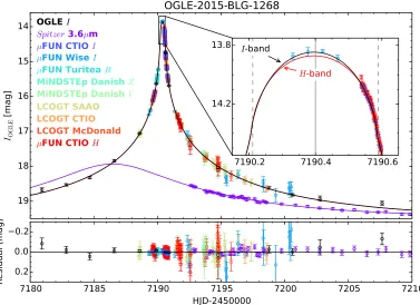
finite source effect is observed, the apparent alignment between the source and the lens must be so perfect that the lens transits the source. Hence, as in a transit, the feature in the light curve is essentially the face of the source resolved in time, and as a result the points offirst and fourth contact can also be seen in the light curve(see, for example, the inset of Figure1). Even in cases in which a finite-source effect is detected, an unambig-uous measurement of the lens mass is still hard to achieve, because the parallax signal is intrinsically small and observa-tionally hard to detect (Gould et al. 2009; Yee et al. 2009; Gould & Yee2013).
The emergence of space-based microlensing has seen improve-ment in the mass measureimprove-ments of microlensing planets (Street et al.2015; Udalski et al.2015b)and binaries(Dong et al.2007; Shvartzvald et al.2015; Zhu et al.2015b). Here we demonstrate with two examples that such space-based observations also increase the probability to measure the mass of single isolated lenses. Within the 170 microlensing events that were selected for
Spitzer observations in the 2015 Spitzer microlensing program
(Gould et al. 2014), we find two single-lens events that show reliable detection of the finite-source effect. Such an effect is observed only in the ground-based data in OGLE-2015-BLG-1268, and only in theSpitzerdata in OGLE-2015-BLG-0763. In both cases, the combination ofSpitzerdata and ground-based data sets provides measurement of parallax. Therefore, mass measure-ments of both microlenses are ensured.
This paper is constructed as follows. The observations of the two events, 1268 and OGLE-2015-BLG-0763, are summarized in Section2; in Section3 we describe the light curve modeling process; the physical interpretations of both events are given in Section4; andfinally in Section5we discuss the interesting findings from these two events, and implications to future space-based microlensing observations.
2. OBSERVATIONS
A general description of the Spitzer observations and ground-based follow-up strategy for the 2015 Spitzer micro-lensing campaign can be found in Yee et al.(2015a)and Street et al. (2015). In brief, events were selected for Spitzer
observations, if (1) they showed or were likely to show significant sensitivity to planets, i.e., events with high peak magnifications (Griest & Safizadeh1998) and/or events with intensive survey observations; and (2) could probably yield parallax measurement. Most Spitzertargets were assigned the default 1-per-day cadence, except that short or relatively high magnification events were given higher cadence. These
42
Sagan Visiting Fellow.
43
NASA Postdoctoral Program Fellow.
44
Sagan Fellow.
45
Royal Society University Research Fellow.
observing protocols were submitted on Monday for observa-tions roughly Thursday through Wednesday for each of the six weeks of the campaign. Ground-based follow-up observations were taken mostly on events that were not heavily monitored by surveys, or when surveys could not observe due to weather or moon passage (e.g., OGLE-2015-BLG-0966, Street et al. 2015). All ground-based data were reduced using standard algorithms (image subtraction/DoPhot), and the
Spitzer data were reduced using the new algorithm presented in Calchi Novati et al. (2015b).
Below we give detailed descriptions of the observations for these two particular events.
2.1. OGLE-2015-BLG-1268
The microlensing event OGLE-2015-BLG-1268 was first alerted by the Optical Gravitational Lens Experiment (OGLE) collaboration through the Early Warning System (EWS) real-time event detection system(Udalski et al.1994; Udalski2003)
on 2015 June 6, based on observations with the 1.4 deg2 camera on its 1.3m Warsaw Telescope at the Las Campanas Observatory in Chile. With equatorial coordinates (RA,
Dec)2000=(17 56 49. 77,h m s - ¢ 21 53 57. 6) and Galactic
coor-dinates(l b, )2000=(7 . 41, 1 . 42 ), this event lies in the OGLE-IV field BLG642 (Udalski et al. 2015a), meaning that it is observed by OGLE with a cadence less than once per two nights, and it was not monitored by the MOA or KMTNet surveys.
Because of the very sparse observations from the survey team, follow-up teams including the Microlensing Follow-Up Network(μFUN, Gould et al.2010), Microlensing Network for the Detection of Small Terrestrial Exoplanets (MiNDSTEp, Dominik et al. 2010) and RoboNet(Tsapras et al.2009)also
observed this event fairly intensively during its peak as seen from Earth, in order to support the Spitzer program and maximize the sensitivity to potential planets(Yee et al.2015a; Zhu et al.2015a). One remarkable feature about these follow-up observations is that the CTIO SMARTS telescope used by the μFUN team could simultaneously obtain H band images whileIband observations were taken(DePoy et al.2003), and these H band observations turned out to be important in characterizing the source star(see next section). Based on the observations taken by 2015 June 16, A.G. issued an alert to the community that this event was deviating from the point-lens point-source model. V.B. later on pointed out that this deviation could befit by a point-lensfinite-source model.
Event OGLE-2015-BLG-1268 was selected for Spitzer
observations on 2015 June 14, i.e.,∼2 days before it reached its peak magnification as seen from Earth. It was classified as a “subjective” event, because it by then did not (in fact, never could)meet the objective criteria set by Yee et al. (2015a). It was selected primarily because it was going to peak with relatively high magnification in the coming week. With a predicted peak magnification Amax,Å >6 (1-σ lower limit)by
the time of selection, this event qualified for bonus observa-tions(Yee et al.2015a), and so was assigned 4-per-day cadence for itsfirst week of observations. Starting from its second week, theSpitzercadence went down to the default value(1-per-day), and this cadence continued for two weeks until it met the criteria set by Yee et al.(2015a)for stopping observations. In total,Spitzerobserved this event 48 times, each with 6 dithered 30s exposures.
[image:3.612.118.495.52.326.2]The data for this event are shown in Figure1. All data sets have been aligned to the OGLE-IVI magnitude according to the best-fit model given in Section3.3.
2.2. OGLE-2015-BLG-0763
This event was first alerted by the OGLE collaboration on 2015 April 22. With equatorial coordinates (RA,
Dec)2000=(17 32 23. 41,h m s - ¢ 29 18 09. 7) and Galactic
coor-dinates (l b, )2000 = - ( 1 . 78, 2 . 25 ), this event lies in the OGLE-IVfield BLG613(Udalski et al.2015a)and is observed by OGLE with once-per-night cadence. It also lies within the region where the new microlensing survey, Korean Microlen-sing Telescope Network(KMTNet, Kim et al.2016)obtained 1-2 observations per day from each of their three 1.6m telescopes as support to theSpitzer campaign. Thus, it is also labeled by the KMTNet team as KMT-2015-BLG-0187.
Events such as this, with OGLE-IV cadence of 1-per-day and lying in non-prime KMTNet fields, are treated by Yee et al.
(2015a)as having low survey coverage in all respects. That is, they are not eligible for objective selection, and once they are selected subjectively, follow-up observations are strongly encouraged. This event hence received a fairly large amount of observations from μFUN RoboNet, and MiNDSTEp, besides the survey observations, although none of these ground-based data showed deviation from the standard point source model.
Event OGLE-2015-BLG-0763 was selected by theSpitzerteam on 2015 May 19, when the Bulge could not yet be seen from
Spitzerdue to its Sun-angle limit. Nevertheless, at that time it was selected as a future Spitzer target in order to achieve high sensitivity to planets. As specified in Yee et al. (2015a) and enacted in Zhu et al.(2015a), when measuring planet sensitivity or detecting planets, only the portion of the light curve taken after the subjective selection of an event may be considered46, in order to isolate any knowledge of the existence of potential planet from the decision making; this is necessary to maintain the objectivity of the sample. The Bulge became accessible toSpitzerstarting from June 6 (HJD¢ º HJD−2450000=7180). Although this event was only assigned 1-per-day cadence, its position, relatively far to the west, made it one of the few targets that could be observed by
Spitzerin the beginning of the Bulge window, and thus it received 8-per-day cadence in the first week. The cadence dropped to 2-per-day as more targets became accessible to Spitzer in the second week. Beginning the third week all targets became accessible toSpitzer, and we devoted the extra time to relatively high magnification events (see Street et al. 2015, for detailed description). Then the cadence for OGLE-2015-BLG-0763 was increased to 8-per-day this week due to its high peak magnification as seen from Earth. The cadence went back to the default one(1-per-day)in the following weeks until it moved out of Spitzer window on HJD¢ =7218. In total, 142 Spitzer
observations were obtained.
The Spitzer data for the six epochs nearest the peak of OGLE-2015-BLG-0763 are affected by saturation and/or nonlinearity. This is quite apparent from the online data presented by Calchi Novati et al. (2015b). For this event, we have therefore re-reduced the data by taking into account the specific characteristics of channel 1 (at 3.6μm) of the IRAC camera. We treat all pixels with counts greater than 70% of the allowed maximum as “corrupted,” i.e., as saturated and/or nonlinear. In addition, all pixels that are interior to corrupted pixels are also treated as corrupted, since the saturation of these pixels can falsely lead to “normal” flux counts. This leads to masking seven to nine pixels for each of these six dithered
images of the epoch closest to peak and to masking up to seven pixels for each of the six dithered images for the remainingfive affected epochs. The remaining pixels(i.e., those below 70% of full well and not interior to corrupted pixels) are treated as normal, since they are essentially unaffected by the nonlinea-rities in neighboring pixels. After the masking of the inner saturated pixels, the fit is therefore carried out in standard fashion. We note that our 70% threshold is conservative with respect to the 90% value in IRAC documentation, and was determined by us empirically from inspection of the raw data and by studying the stability of the photometry PRF fitting solution.47
The data for this event are shown in Figure2. Again, all data sets have been aligned to the OGLE-IVImagnitude according to the best-fit model given in Section3.4.
3. LIGHT CURVE ANALYSES
3.1. Modeling Process
For each event, we perform a Markov Chain Monte Carlo analysis to find the best-fit parameters and the associated probability density functions using the emcee ensemble sampler (Foreman-Mackey et al. 2013). The formalism to incorporate the finite-source effect in the single-lens case is given in Yoo et al.(2004). For each microlensing event, there will be six event parameters: time of maximum magnification as seen from Eartht0, the impact parameter in the absence of parallax as seen from Earth u0, the event timescale tE, the
source radius scaled to the angular Einstein radiusρ, and the two components of microlens parallax along the north and east directionpE,NandpE,E. For each data set on that event, there are
two flux parameters (fs, fb). In addition, we have two limb-darkening coefficients(q˜1,l,q˜2,l)described in the next section. If these are also set free, there are two additional parameters for each bandpass.
For each event that is investigated below, we report the six event parameters as well as the blending fraction in the OGLE-IVIband. This blending fraction, defined as fb (fs+fb), can be used to distinguish between degenerate models, as we will see below.
3.2. Limb Darkening Effect
For the present cases, especially OGLE-2015-BLG-1268, many of our observations were taken when the alignment between the source and the lens was closer than roughly the scaled source size ρ, so the generally adopted linear limb-darkening law is not adequate. Therefore, we choose the two-parameter square root limb darkening law
( )m = ¯ - G - m - L - m ( )
l l⎡ l⎜ ⎟ l⎜ ⎟
⎣⎢
⎛
⎝ ⎞⎠ ⎛⎝ ⎞⎠
⎤ ⎦⎥
S S 1 1 3
2 1
5
4 , 3
in whichμis the cosine of the angle between the line of sight and the emergent intensity, and Gl and Ll are the limb-darkening
coefficients at wavelengthλ. Because of our requirement that the totalflux,Ftot,l=pq2S¯l, should be conserved for a given source
angular sizeq, Equation(3)differs from the standard square root
limb-darkening law described by (cl,dl) in Diaz-Cordoves & Gimenez (1992). The transformations between limb-darkening
46
Unless it is later found to meet objective selection criteria.
47
We have tested that the results remain the same even though higher threshold values(up to 90%)are used.
coefficients (G Ll, l) and (cl,dl) can be found in Fields
et al.(2003).
In cases in which very little knowledge of the source star can be obtained otherwise, one may want to fit for (G Ll, l).
However, simply leaving (G Ll, l)free will very likely lead to unphysical stellar brightness profiles. Therefore, we reparame-terize the limb-darkening coefficients(G Ll, l)using the method
proposed by Kipping(2013),
˜ lº G + L( l l) ( )
q1, 2, 4
˜
( ) ( )
º L
G + L
l l
l l
q 7
12 . 5
2,
The inverse transformation is given by
˜ ˜ ( )
G =l q l⎜⎛⎝1- 12q l⎟⎞⎠
7 , 6
1, 2,
˜ ˜ ( )
L =l 12 q lq l
7 1, 2, . 7
As Kipping (2013) has shown, uniform samplings in the interval [0, 1] for both q˜1,l and q˜2,l can ensure physically meaningful stellar intensity profiles48 as well as being efficient.49
3.3. OGLE-2015-BLG-1268
In the case of OGLE-2015-BLG-1268, because we were unable to fully understand the source star with only photometric data(see Section4.1), we alsofit for the limb-darkening coefficients. Since
only theIandHband data were relevant when thefinite-source effect is prominent, we only set the limb-darkening coefficients of these two bands free. Furthermore, since the Spitzer data only captured the falling tail of the light curve, a constraint on the source flux in the Spitzer3.6μm band (Lspitzer) is necessary in order to better measure the parallax (Calchi Novati et al.2015a, 2015b). This is done by conducting a color–color regression betweenI−HandI-Lspitzer using stars with color
and magnitude similar to the clump.
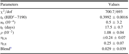
Our best-fit model to this event is shown in Figure1, and
best-fit parameters with 1-σintervals are given in Table1. Note that in Figure 1, the Hband model shows deviations from the Iband model, which are obvious on the top and still noticeable at the limb. Characterizing events via such deviations for point-lens
(Gould & Welch 1996) and planetary (Gaudi & Gould 1997)
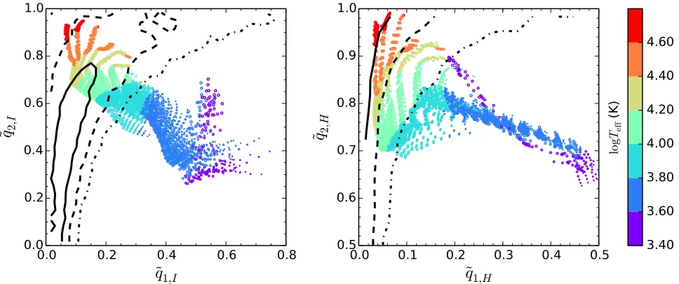
events was the original motivation for building the dichroic ANDICAM camera(DePoy et al.2003). We show in Figure3the
c
D 2=1, 4 and 9 contours between( ˜ ˜ ) l l
q1, ,q2, on the top of the
theoretical values from Claret(2000). The constraint on theIband limb-darkening coefficients ( ˜q1,I,q˜ )2,I favors hot stars
(Teff8000K)at 2-σlevel, and this is consistent with the less
constrainedHband limb-darkening coefficients.
Since the impact parameter as seen from Earth is extremely small(indeed, consistent with zero)compared to the that seen from Spitzer, the generic four-fold degeneracy in single-lens events collapses to two-fold, i.e., to a degeneracy only in the direction of pE (and not its magnitude). However, this
degeneracy in direction has no effect on the mass and distance measurement(Gould & Yee 2012).
3.4. OGLE-2015-BLG-0763
[image:5.612.120.493.57.326.2]For OGLE-2015-BLG-0763, we adopt the limb-darkening coefficients that correspond to the well characterized source
Figure 2.Ground-based andSpitzerdata and best-fit model light curves for OGLE-2015-BLG-0763. Thefinite source effect is only seen in theSpitzerdata. Ground-based data points with uncertainties>0.2mag are suppressed in thefigure to avoid clutter, but are included in the modeling.
48
Positive intensity everywhere, and monotonically decreasing intensity from the center to the limb.
49
[image:5.612.45.294.465.581.2](see Section 4.2), so that only event parameters and flux parameters are free in the modeling. The best-fit model is shown in Figure2, and the best-fit parameters together with 1-σ intervals for the two adopted solutions,(+ -, )and(- +, ), are given in Table 2. Parameters of the other possible solutions, i.e.,(+ +, )and(- -, )solutions, are similar except that only an upper limit on the source size,r0.01atDc2 =4 or 2-σ
level, can be obtained, meaning that the finite-source effect is not securely detected. Nevertheless these two solutions are rejected, partly because they are disfavored byDc2=15, and
also because the derived physical parameters result in inconsistency with observations(see Section4.2).
The two adopted solutions have different parallax vectorpE
but similar amplitude pE, as is shown in Table 2. As in the
previous case, for the purpose of mass and distance determination this means that the four-fold degeneracy is also broken here. We show in Section5that this is not coincidental, but is rather almost inevitable for mass measurements of single-lens events with space-based observations.
4. PHYSICAL INTERPRETATIONS
4.1. OGLE-2015-BLG-1268L: A Brown Dwarf(BD)in the Inner Disk
The extinction in the region where this event lies is so high that the routine OGLE-IVVband images are not deep enough to resolve the red giant clump in the Bulge. In order to determine the color and magnitude of the source star following the standard routine (Yoo et al. 2004), we then construct an
I−H versus I color–magnitude diagram (CMD) in the following way: we obtain OGLE-IV I band magnitudes for stars within2¢separation from the event, and cross-match to the VISTA Variables in the Vía Láctea Survey (VVV, Saito et al.2012)to obtain theirHband magnitudes. The position of the source star on this CMD is found to be
(I-H I, )s =(2.9970.003, 19.540.04 ,) ( )8
in which Is comes directly from the modeling and Hs is determined by transforming the CTIO instrumental H-band sourceflux that is derived from the model to the standard VVV system using comparison stars. The centroid of the red clump on this CMD is at
(I-H I, )cl =(4.000.02, 17.78 0.05 .) ( )9
The CMD for this event with the positions of the source and the clump centroid indicated is shown on the left panel of Figure4.
Comparing to the dereddened color and magnitude of the clump at this particular direction,(I-H I, )cl,0 =(1.29, 14.23) (Bensby et al. 2013; Nataf et al.2013), we determine the extinction and reddening to beAI=3.6 and E I( -H)=2.7, respectively. If all of this extinction applies to the source star, the dereddened source will have
(I-H I, )s,0=(0.290.02, 15.99 0.08 .) (10)
and MI=1.65. These values suggest the source star is a late A/early F dwarf(Bessell & Brett1988). Such stars are rare in the Bulge(Bensby et al.2013; Poleski et al.2014). In principle, one could not exclude the possibility that the source might not lie behind the same amount of dust as the clump does, so that an intrinsically redder and therefore dimmer but closer source star is also allowed by this CMD analysis. However, the limb-darkening coefficients from our light curve modeling (see Figure3) also suggest that the source star hasTeff8000K
when compared to the theoretical values given by Claret
(2000). Therefore, we conclude that the source star is an A-type dwarf in the Bulge(or at least at a roughly similar distance as the Bulge).
We then use the dereddened source color and magnitude to derive the angular radius of the source star. Boyajian et al.
(2014) provide the following relation to estimate the stellar angular diameter based on the dereddened I−Hcolor and I
magnitude
( ) ( )
= + -
-d a a I H I
log 0 1 0.2 , 11
with a0=0.530260.00077, a1=0.365950.00079.
Adopting the above dereddened color and magnitude of the source, wefind that the source angular radius is
( ) ( )
q = 1.37 0.10 mas. 12
The uncertainty here is dominated by the7.4% scatter in the color-surface brightness relation(Equation(11)).
When combined with the source radiusr=0.01080.0005, it yieldsqE=0.1270.009mas. Given the microlens parallax
measurement pE=0.350.0450 We then find the lens mass
and the lens-source relative parallax
( ) ( )
( )
p
= =
M 0.045 0.007 M ; 0.044 0.006 mas,
13
L rel
and then(adoptingDS=81kpc), a lens distance
( ) ( )
=
DL 5.9 1.0 kpc. 14
That is, a BD in the inner Galactic disk.
The lens-source relative proper motion, mrel=2.65
-0.20 mas yr 1, is more typical of Bulge lenses (m ~
rel
-4 mas yr 1) than disk lenses (m ~7 mas yr
-rel 1). However,
[image:6.612.42.296.74.181.2]this value is certainly not inconsistent with a disk lens for two reasons. First, the higher proper motions typical of disk lenses
Table 1
Best-fit Parameters of OGLE-2015-BLG-1268
Parameters Values
c2/dof 700.7/693
t0(HJD′−7190) 0.3992±0.0016
u0(10-4) 0.5±3.2
tE(days) 17.5±0.7
ρ(10-2) 1.08±0.04
pE,N ±0.24±0.07
pE,E 0.25±0.07
Blenda 0.029±0.039
Note. a
Blending fraction in the OGLE-IVIband.
50
Note that the uncertainty onpEis smaller than the uncertainty on eitherpE,N
orpE,E(see Table1)because of the anti-correlation betweenpE,NandpE,E. This
anti-correlation emerges due to the constraint on the sourceflux inLspitzerband.
In particular, Gould & Yee(2012)showed that for high-magnification events
(as seen from Earth), pE can be determined from a single space-based
observation taken at the ground-based peak (plus one additional late-time observation), provided the space-based sourceflux is known. In this case, there would be perfect knowledge of the magnitude ofpEand perfect ignorance of
its direction. While the observations of OGLE-2015-BLG-1268 do not satisfy this condition(see Figure1), essentially the same logic applies.
come from the fact that the Sun and the disk lens partake of the same relatively flat Galactic rotation curve, while Bulge sources are on average not moving in the frame of the Galaxy. Hence, disk lenses tend to have similar proper motions as SgrA*. However, in the present case, the source may also be in the disk as indicated by the fact that it is likely to be an A star. If so, it would partake of the same flat rotation curve, which then naturally leads to a low proper motion. Second, one of the two solutions(withpE,N>0)is approximately in the direction
of Galactic rotation, so that the Bulge source would have to be moving at just mS~4 mas yr-1 in the direction of Galactic
rotation(i.e.,1.3s)to account for the observed relative proper motion.
The Galactic coordinates of the event,(l b, )=(7 . 41, 1 . 42 ), provide a further indication that the source may be in the disk. That is, even if the source were at roughly the Galactocentric distance, it would lie just ∼200 pc from the plane, which is significantly populated by late A/early F stars. Moreover, at this longitude, disk stars account for a significantly larger fraction of stars at these distances than is the case for typical microlensing fields nearl~0. Thus, this possibility must be taken seriously.
Now, if the source were in the disk, this would not in any way affect eitherMLorprel, provided that the source lies behind
the same dust column as the clump. This is because the estimate of q (and so qE) depends only on the dereddened
color and magnitude of the source and not its distance. However, given the various evidences favoring a disk source, as well as the low Galactic latitude of the event, we must consider the possibility that the source does in fact lie in front of at least some of the dust.
Hence, we develop a more robust way to estimate the lens mass that does not require the source lying behind all the dust. According to the color-surface brightness relation ( Equa-tion (11)), one can write the angular source radius q (and
furtherML)in terms of the dereddened source color(I-H)s,0
and magnitude Is,0. If the reddening law derived from the red
clump,RIH =A E II ( -H)=1.33, also applies to the source
star, we can express(I-H)s,0andIs,0in terms of(I-H)s,Is,
and a single parameterη,
( ) ( ) ( ) ( )
h
h
= +
- = - +
-I I A
I H I H E I H
,
. 15
I
s,0 s,0,naive
s,0 s,0,naive
Hereηis the fraction of total extinction of dust lying behind the source (and in front of the clump), while Is,0,naive and
(I-H)s,0,naive are the values we derived above under the
naive assumption thath =0. Combining Equations (11) and
(15)with the observed RIH =1.33and E I( -H)=2.7, one finds that as one variesη,q changes by
( )( ) ( )
q h h
Dlog = E I-H a1-0.2RIH =0.27 . 16
Thus in particular, our conclusion that the best estimate for the lens mass is in the BD regime (M<0.08M) rests on the
[image:7.612.66.550.51.254.2]assumption that h<log 0.08 0.045 0.27( ) =0.86. This is very likely simply because nearby sources are extremely rare in microlensing due to low optical depth. Nevertheless, it would be of interest to definitively resolve this issue. This could be done simply by identifying the stellar type of the source via a low-resolution spectrum. This would remove the uncertainty due to the location of the source with respect to the dust. It
Figure 3.TheDc2=1, 4 and 9 constraints(solid, dashed and dotted–dashed curves, respectively)on the limb-darkening coefficients in theIband(left)andHband (right)in the case of OGLE-2015-BLG-1268. Open circles are theoretical values taken from Claret(2000)after the transformation from(c,d)to( ˜q q1, ˜ )2, and they are
color coded with the stellar effective temperature. The constraints on limb-darkening coefficients effectively rule out a source withTeff<8000K.
Table 2
Best-fit parameters of OGLE-2015-BLG-0763
Parameters (+ -, ) (- +, )
c2/dof 1469.8/1463 1468.7/1463
t0(HJD′−7189) 0.038±0.005 0.045±0.005
u0(10-2) 5.92±0.06 −5.99±0.06
tE(days) 33.09±0.24 32.78±0.25 ρ(10-2) 2.18±0.05 2.17±0.05 pE,N −0.0684±0.0007 0.0707±0.0008
pE,E 0.0174±0.0002 0.0083±0.0002
Blenda −0.035±0.010 −0.049±0.012
Note.The other two possible solutions,(+ +, )and(- -, ), are disfavored by
c
D 2=15, and haver0.01(2-σlimit)that is inconsistent with the blend
constraint(see Section4).
a
[image:7.612.43.294.326.432.2]would also permit one to determineqwithout appealing to the
detailed modeling of limb-darkening coefficients from the light curve(Section3.3).
4.2. OGLE-2015-BLG-0763L: An M-type Main-sequence Star in the Inner Disk
We first characterize the source of OGLE-2015-BLG-0763 using the method of Yoo et al. (2004). Combining the light curve modeling and a linear regression of OGLE-IVVband on
Ibandflux during the event yield(V-I I, )s=(3.25, 17.27). The clump centroid in thisV−IversusICMD(see the right panel of Figure 4) is found at (V-I I, )cl=(3.00, 16.89). After the correction of OGLE-IV non-standard V band (Zhu et al. 2015b), and combining with the dereddened color
(Bensby et al.2013)and magnitude(Nataf et al.2013)of the clump at this direction, we derive the color and magnitude of the dereddened source to be (V-I I, )s,0=(1.29, 14.78). Thus, the source is a giant star in the Bulge. We then convert fromV−ItoV−Kusing the empirical color–color relations of Bessell & Brett (1988), apply the color-surface brightness relation of Kervella et al. (2004), andfind the source angular radius
( )
q =6.30.4 as.m 17
The uncertainty here has taken into account the uncertainty in centroiding the clump I-band magnitude in the CMD
(∼0.05 mag) and the derivation of the intrinsic source color
(0.05 mag, Bensby et al.2013).
Given the source sizer=0.02180.0007from light curve modeling,51 this indicates an angular Einstein radius qE=
0.288 0.020mas. We then combine this with the microlens
parallax parameter pE=0.07090.0010 and find the lens
mass and distance
( )
= =
ML 0.50 0.04M , DL 6.9 1.0 kpc. 18
In derivingDL we have assumed a Bulge source(DS=81
kpc), which is very likely the case given the location of this event. Given the timescale tE=32.90.3 days, the
lens-source relative proper motion is mrel=3.200.25 mas/yr, and it is almost due the north/south direction(pE,E∣pE,N∣).
As is mentioned in Section 3.4, the other two solutions (+ +, ) and (- -, ) are disfavored by Dc2=15 and only
provide upper limit of 0.01 on ρ. Regardless of the c2
argument, if this set of solutions were correct, the lens would have mass1.0Mand distance 6 kpc. First of all, more massive
stars are intrinsically rarer. Furthermore, a 1Mmain-sequence
star would be 12% as bright as the source star, and therefore contribute 11% of the total baselineflux. This contradicts the fact that slightly negative blending is detected in this event.52 Therefore, these two solutions are discarded.
5. DISCUSSION
The mass determination of isolated microlenses requires measurements of at least two of the three important microlen-sing parameters: the angular Einstein radiusqE, the microlens
parallaxpE, and the lensflux. Among them, measuring the lens
flux requires the lens to be luminous, so that it will not work for faint or dark lenses, although it may see broad applications in future space-based microlensing experiments (Yee 2015). Therefore, measuringqE and pE together is the only method
that works for all types of objects.
In this work, we report on the mass and distance measure-ments of two single-lens events from our 2015 Spitzer
microlensing program. The finite-source effect is detected in the ground-based data in OGLE-2015-BLG-1268, and in the
[image:8.612.67.549.53.280.2]Spitzer data in OGLE-2015-BLG-0763, ensuring measurement
Figure 4.The color–magnitude diagrams(CMD)used to characterize the source of OGLE-2015-BLG-1268(left)and OGLE-2015-BLG-0763(right). In both cases, the centroid of the red clump is indicated by afilled red square, and the position of the source is marked by a blue asterisk.
51
Here we combine the results of (+ -, ) and (- +, ) solutions, and the uncertainty takes into account the difference between both solutions and the uncertainty of each solution.
52
The adopted solution, a 0.5Mstar at 6.9 kpc, cannot produce a negative
blending either, but this solution is much more plausible given the fact that various effects can lead to slightly negative blending(Smith et al.2007).
of the angular Einstein radius qE. The microlens parallax
parameterpEis measured from a combinedfit to the ground- and
space-based data. We find that the lens of OGLE-2015-BLG-1268 is very likely a BD, and probably a 45MJBD at 5.9 kpc if
the source star is inside the galactic Bulge. The lens of OGLE-2015-BLG-0763 is a 0.5Mstar at 6.9 kpc.
The result that at least two53single-lens events out of the 170 monitored events in the 2015 Spitzer program yield mass measurements was unexpected, but turns out to be reasonable. To measure the mass of isolated microlenses by combiningqE
andtE, one needs to detect thefinite-source effect and measure
the microlens parallax. The first is approximately a geometric probability for the lens to“transit”the source star, which is of order ρ54, and the second, in the case of two-observatory parallax method(Refsdal1966; Gould1994b,1997), is limited mostly by the projected separation between the two observa-tories D^. In order to measure the parallax, the two
observatories should both be able to detect the same event, but should each see (slightly) different light curves. In the presence of thefinite-source effect, this provides the following constraints on the projected Einstein radiusr˜Eºau pE,
˜ ( )
r
^ ^
D rE 50D . 19
where in the second inequality we have assumed typical photometric uncertainty (2%) during peak (Gould & Yee
2013). For a lens with mass ML, the above inequalities then
provide upper and lower limit on the lens distance for which microlens parallax is detectable (assuming Bulge sources)
( )
q p k
^ ^
⎛ ⎝ ⎜ ⎞
⎠ ⎟
D M D
au 50
au
. 20
rel L
2
For terrestrial parallax (D^~RÅ), the upper constraint onprel
is almost always satisfied unless the lens is extremely low-mass or extremely nearby. The combined constraint thus suggests that only relatively nearby (DL2.5kpc) lenses can be
probed by terrestrial parallax, and since the lensing probability of such stars is quite low, the overall probability to measure isolated lens masses through this channel is extremely low. This has been shown in Gould & Yee (2013), in which they found an event rate ∼1.6 Gyr−1. Observationally, in the era prior to the Spitzer microlensing campaign, only two single-lens microsingle-lensing events yielded mass measurements ( OGLE-2007-BLG-224 and OGLE-2008-BLG-279, Gould et al.2009; Yee et al.2009)in this way, although more than 10,000 events were discovered and at least four thousand of them were monitored as intensively as Spitzerevents.55
Equation(20)also shows that in a Spitzer-like microlensing program(D^~1 au), the parallax parameter is measurable for
the majority of microlensing events. This has been proved by the 2014 & 2015 Spitzer microlensing programs (Calchi Novati et al. 2015a, 2015b). In addition, the lens-source relative trajectory is most often very different as seen from Earth and from the satellite. This means that the probability to detect the
finite-source effect in single-lens events is almost doubled. Thus, the overall probability to make mass measurements of isolated microlenses forSpitzeris2á ñr u0,max, whereá ñ ~r 0.005is the
average source size normalized to the Einstein radius forSpitzer
events, andu0,max »0.3is set as one of the criteria for selecting
events(Yee et al.2015a). This theoretical estimate(3.3%)agrees with the apparent frequency of such events (3 170=1.8%)
reasonably well, with the factor of∼2 difference likely due to the incomplete coverage of Spitzer data in some events. Hence, space-based microlensing experiments such as Spitzer and
Kepler (Gould & Horne 2013; Henderson et al. 2015) can significantly increase the probability to measure the mass of isolated microlenses, besides their primary goal of detections and statistical studies of planets. Furthermore, because the impact parameter of the observatory that shows thefinite-source effect must be close to zero, the generic four-fold degeneracy in single lens cases is effectively broken(Gould & Yee2012).
Measuring the mass of isolated microlenses is of great scientific interest. Gould (2000) estimated that ~20% of all Galactic microlensing events are caused by stellar remnants, and specifically that ~1% are due to stellar mass black holes. In addition, there exists a population of probably unbound planet-mass objects that are almost twice as common as main-sequence stars(Sumi et al.2011). These isolated stellar remnants and free
floating planets(FFPs)can only be probed by microlensing, and our work shows that space-based observations can significantly enhance the probability to definitely measure their masses.
The future of detecting dark or extremely faint isolated objects via microlensing is promising. In addition to Spitzer, the re-proposed Kepler mission (K2, Howell et al. 2014) is going to continuously monitor a 4 deg2microlensingfields for
∼70 days in its campaign 9, which provides so far a unique chance to probe especially the FFP population(Gould & Horne
2013; Henderson et al.2015). Future space-based microlensing missions such as the Wide-field InfraRed Survey Telescope
(Spergel et al.2015)and possibly Euclid(Penny et al. 2013), once combined with a simultaneous ground-based telescope network, will significantly increase the sensitivities to espe-cially FFPs with even lower masses(Zhu & Gould2016).
Work by WZ, SCN and AG was supported by JPL grant 1500811. WZ and AG also acknowledge support by NSF grant AST-1516842. Work by JCY was performed under contract with the California Institute of Technology (Caltech)/Jet Propulsion Laboratory (JPL) funded by NASA through the Sagan Fellowship Program executed by the NASA Exoplanet Science Institute. The Spitzer Team thanks Christopher S. Kochanek for graciously trading us his allocated observing time on the CTIO 1.3 m during the Spitzer campaign. The OGLE project has received funding from the National Science Centre, Poland, grant MAESTRO 2014/14/A/ST9/00121 to au. This work is based in part on observations made with the Spitzer
Space Telescope, which is operated by the Jet Propulsion Laboratory, California Institute of Technology under a contract with NASA. Work by CH was supported by Creative Research Initiative Program (2009-0081561) of National Research Foundation of Korea. This research has made the use of the
53The single-lens event OGLE-2015-BLG-1482 also shows finite-source
effect as seen fromSpitzer(Chung, S-J. et al. 2016, in preparation).
54
The observational bias tends to enhance the probability of detecting such finite-source effects in single-lens events that are caused by faint dwarf source stars. See Zhu & Gould(2016)for more discussions.
55
KMTNet telescopes operated by the Korea Astronomy and Space Science Institute (KASI), and was supported by KASI grant 2016-1-832-01. This work makes use of observations from the LCOGT network, which includes three SUPAscopes owned by the University of St Andrews. The RoboNet programme is an LCOGT Key Project using time allocations from the University of St Andrews, LCOGT and the University of Heidelberg together with time on the Liverpool Telescope through the Science and Technology Facilities Council (STFC), UK. This research has made use of the LCOGT Archive, which is operated by the California Institute of Technology, under contract with the Las Cumbres Observatory. KH acknowledges support from STFC grant ST/M001296/1. This project is partly supported by the Strategic Priority Research Program “The Emergence of Cosmological Structures”of the Chinese Academy of Sciences, Grant No. XDB09000000(SM and SD). MPGH acknowledges support from the Villum Foundation. NP acknowledges funding by the Gemini-Conicyt Fund, allocated to the project No. 32120036. Based on data collected by MiNDSTEp with the Danish 1.54 m telescope at the ESO La Silla observatory. Operation of the Danish 1.54 m telescope at ESOs La Silla observatory was supported by The Danish Council for Independent Research, Natural Sciences, and by Centre for Star and Planet Formation. The MiNDSTEp monitoring campaign is powered by ARTEMiS (Automated Terrestrial Exoplanet Microlensing Search, Dominik et al.2008). DMB acknowledges support from NPRP grant # X-019-1-006 from the Qatar National Research Fund (a member of Qatar Foundation). GD acknowledges Regione Campania for support from POR-FSE Campania 2014-2020. OW and JS acknowledge support from the Communauté francaise de Belgique’ Actions de recherche concertées’Académie universitaire Wallonie-Europe.
REFERENCES
Bensby, T., Yee, J. C., Feltzing, S., et al. 2013,A&A,549, A147 Bessell, M. S., & Brett, J. M. 1988,PASP,100, 1134
Boyajian, T. S., van Belle, G., & von Braun, K. 2014,AJ,147, 47 Calchi Novati, S., Gould, A., Udalski, A., et al. 2015a,ApJ,804, 20 Calchi Novati, S., Gould, A., Yee, J. C., et al. 2015b,ApJ,814, 92 Claret, A. 2000, A&A,363, 1081
DePoy, D. L., Atwood, B., Belville, S. R., et al. 2003,Proc. SPIE,4841, 827 Diaz-Cordoves, J., & Gimenez, A. 1992, A&A,259, 227
Dominik, M., Horne, K., Allan, A., et al. 2008,AN,329, 248
Dominik, M., Jørgensen, U. G., Rattenbury, N. J., et al. 2010,AN,331, 671 Dong, S., Udalski, A., Gould, A., et al. 2007,ApJ,664, 862
Fields, D. L., Albrow, M. D., An, J., et al. 2003,ApJ,596, 1305
Foreman-Mackey, D., Hogg, D. W., Lang, D., & Goodman, J. 2013,PASP, 125, 306
Gaudi, B. S., & Gould, A. 1997,ApJ,486, 85 Gould, A. 1992,ApJ,392, 442
Gould, A. 1994a,ApJL,421, L71 Gould, A. 1994b,ApJL,421, L75 Gould, A. 1997,ApJ,480, 188 Gould, A. 2000,ApJ,535, 928 Gould, A. 2013,ApJL,763, L35
Gould, A., Carey, S., & Yee, J. 2014, spitz prop,11006 Gould, A., Dong, S., Gaudi, B. S., et al. 2010,ApJ,720, 1073 Gould, A., & Horne, K. 2013,ApJL,779, L28
Gould, A., & Loeb, A. 1992,ApJ,396, 104
Gould, A., Udalski, A., Monard, B., et al. 2009,ApJL,698, L147 Gould, A., & Welch, D. L. 1996,ApJ,464, 212
Gould, A., & Yee, J. C. 2012,ApJL,755, L17 Gould, A., & Yee, J. C. 2013,ApJ,764, 107 Griest, K., & Safizadeh, N. 1998,ApJ,500, 37
Henderson, C. B., Penny, M., Street, R. A., et al. 2015, arXiv:1512.09142 Honma, M. 1999,ApJL,517, L35
Howell, S. B., Sobeck, C., Haas, M., et al. 2014,PASP,126, 398
Kervella, P., Thévenin, F., Di Folco, E., & Ségransan, D. 2004,A&A,426, 297 Kim, S.-L., Lee, C.-U., Park, B.-G., et al. 2016, JKAS,49, 37
Kipping, D. M. 2013,MNRAS,435, 2152 Mao, S., & Paczynski, B. 1991,ApJL,374, L37
Nataf, D. M., Gould, A., Fouqué, P., et al. 2013,ApJ,769, 88 Paczynski, B. 1986,ApJ,304, 1
Penny, M. T., Kerins, E., Rattenbury, N., et al. 2013,MNRAS,434, 2 Poleski, R., Skowron, J., Udalski, A., et al. 2014,ApJ,795, 42 Refsdal, S. 1966,MNRAS,134, 315
Saito, R. K., Hempel, M., Minniti, D., et al. 2012,A&A,537, A107 Shvartzvald, Y., Udalski, A., Gould, A., et al. 2015,ApJ,814, 111 Smith, M. C., Woźniak, P., Mao, S., & Sumi, T. 2007,MNRAS,380, 805 Spergel, D., Gehrels, N., Baltay, C., et al. 2015, arXiv:1503.03757 Street, R. A., Udalski, A., Calchi Novati, S., et al. 2016,ApJ,819, 93 Sumi, T., Kamiya, K., Bennett, D. P., et al. 2011,Natur,473, 349 Tsapras, Y., Street, R., Horne, K., et al. 2009,AN,330, 4 Udalski, A. 2003, AcA,53, 291
Udalski, A., Szymanski, M., Stanek, K. Z., et al. 1994, AcA,44, 165 Udalski, A., Szymański, M. K., & Szymański, G. 2015a, AcA,65, 1 Udalski, A., Yee, J. C., Gould, A., et al. 2015b,ApJ,799, 237 Witt, H. J., & Mao, S. 1994,ApJ,430, 505
Yee, J. C. 2015,ApJL,814, L11
Yee, J. C., Gould, A., Beichman, C., et al. 2015a,ApJ,810, 155 Yee, J. C., Udalski, A., Calchi Novati, S., et al. 2015b,ApJ,802, 76 Yee, J. C., Udalski, A., Sumi, T., et al. 2009,ApJ,703, 2082 Yoo, J., DePoy, D. L., Gal-Yam, A., et al. 2004,ApJ,603, 139 Zhu, W., & Gould, A. 2016, arXiv:1601.03043
Zhu, W., Gould, A., Beichman, C., et al. 2015a,ApJ,814, 129 Zhu, W., Udalski, A., Gould, A., et al. 2015b,ApJ,805, 8