Development of Predictive QSPR Model of the First Reduction Potential from a Series of Tetracyanoquinodimethane (TCNQ) Molecules by the DFT (Density Functional Theory) Method

https://www.scirp.org/journal/cc ISSN Online: 2332-5984

ISSN Print: 2332-5968

DOI: 10.4236/cc.2019.74009 Oct. 22, 2019 121 Computational Chemistry

Development of Predictive QSPR Model of the

First Reduction Potential from a Series of

Tetracyanoquinodimethane (TCNQ) Molecules

by the DFT (Density Functional Theory) Method

Fatogoma Diarrassouba

, Mawa Koné

, Kafoumba Bamba

, Yafigui Traoré

,

Mamadou Guy-Richard Koné

, Edja Florentin Assanvo

1_{Laboratoire de Thermodynamique et de Physico-chimie du Milieu, UFR-SFA, Université Nangui Abrogoua, Abidjan,} Côte d’Ivoire

2_{Laboratoire de Chimie Organique et des Substances Naturelles, UFR-SSMT, Université Félix Houphouët Boigny, Abidjan,} Côte d’Ivoire

Abstract

In this work, which consisted to develop a predictive QSPR (Quantitative Structure-Property Relationship) model of the first reduction potential, we were particularly interested in a series of forty molecules. These molecules have constituted our database. Here, thirty molecules were used for the training set and ten molecules were used for the test set. For the calculation of the de-scriptors, all molecules have been firstly optimized with a frequency calcula-tion at B3LYP/6-31G(d,p) theory level. Using statistical analysis methods, a predictive QSPR (Quantitative Structure-Property Relationship) model of the first reduction potential dependent on electronic affinity (EA) only have been developed. The statistical and validation parameters derived from this model have been determined and found interesting. These different parameters and the realized statistical tests have revealed that this model is suitable for pre-dicting the first reduction potential of future TCNQ (tetracyanoquinodime-thane) of this same family belonging to its applicability domain with a 95% confidence level.

Keywords

Tetracyanoquinodimethane, First Reduction Potential, QSPR, Statistical Analysis

1. Introduction

Conjugated simple organic molecules carrying both electron donors and

accep-How to cite this paper: Diarrassouba, F., Koné, M., Bamba, K., Traoré, Y., Koné, M.G.-R. and Assanvo, E.F. (2019) Devel-opment of Predictive QSPR Model of the First Reduction Potential from a Series of Tetracyanoquinodimethane (TCNQ) Mo-lecules by the DFT (Density Functional Theory) Method. Computational Chemi-stry, 7, 121-142.

https://doi.org/10.4236/cc.2019.74009

Received: September 5, 2019 Accepted: October 19, 2019 Published: October 22, 2019

Copyright © 2019 by author(s) and Scientific Research Publishing Inc. This work is licensed under the Creative Commons Attribution International License (CC BY 4.0).

http://creativecommons.org/licenses/by/4.0/

DOI: 10.4236/cc.2019.74009 122 Computational Chemistry tors have recently attracted a lot of attention because of their various and inter-esting properties. Non-linear optical properties [1], molecular electronic devices [2], artificial photosynthesis models [3] and solvatochromic effects [4] are among their potential applications.

Intramolecular electron transfer processes are one of the main topics of cur-rent interest in physic organic chemistry [5], particularly regarding tetracyano-quinodimethane (TCNQ)-based charge transfer complexes. In fact, TCNQ is an organic electron acceptor with a high electron affinity [6] [7] [8]. This electron acceptor can react according to an oxidation-reduction process with electron donors to form charge transfer complexes that display electrical properties and various applications. Indeed, it has been used for the synthesis of a large number of charge transfer compounds that have been widely explored as molecular elec-tronics building blocks [9] [10], non-linear optics [11] and organic semiconduc-tors [12] [13]. Existing TCNQ molecules have generally exhibited exemplary re-dox properties. Improving their properties and finding molecules with even bet-ter properties is therefore a challenge for scientific research. However, in the syn-thesis of these complexes, the objective of organic chemists is to synthesize ther-modynamically stable radical species, which is not an easy task. Also, the two molecules constituting the charge transfer complex must have moderate donor and acceptor powers [14]. Under these conditions, the use of alternative me-thods for experimentation becomes essential. Among these, QSPR (Quantitative Structure-Property Relationships) methods are of great interest and even rec-ommended according to new regulations [15] [16]. They make it possible to de-velop mathematical models linking physico-chemical properties with molecular structure. They either explain the origin of these properties or predict them for the molecules whose experimental data are not available. Quantum chemistry provides access to a large number of descriptors through its different methods.

The objective of this work is to develop a predictive QSPR model of the first reduction potential from a series of TCNQ molecules using quantum descriptors, to explain and predict the first reduction potential of the future TCNQ mole-cules of this same family belonging to its applicability domain.

2. Computational Details

2.1. Training Set and Test Set

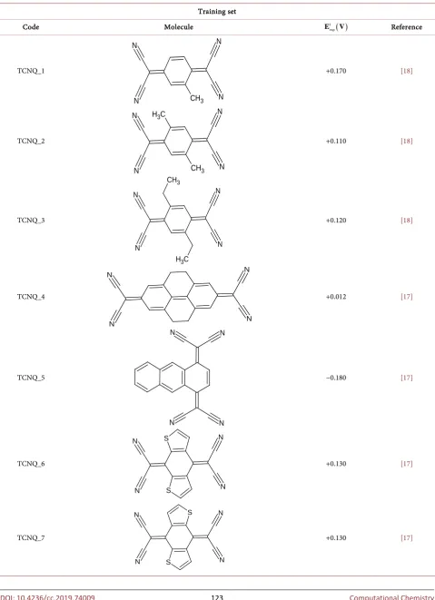
DOI: 10.4236/cc.2019.74009 123 Computational Chemistry Table 1. Series of studied tetracyanoquinodimethane (TCNQ) molecules.

Training set

Code Molecule 1 ( )

exp

E V Reference

TCNQ_1 +0.170 [18]

TCNQ_2 +0.110 [18]

TCNQ_3 +0.120 [18]

TCNQ_4 +0.012 [17]

TCNQ_5 −0.180 [17]

TCNQ_6 +0.130 [17]

TCNQ_7 +0.130 [17]

N

N N

N

CH₃

N

N N

N

CH₃ C

H₃

N

N N

N

C H₃ CH₃

N N N

N

N N

N N

N

N N

N S

S

N

N N

N S

DOI: 10.4236/cc.2019.74009 124 Computational Chemistry Continued

TCNQ_8 −0.470 [17]

TCNQ_9 -0.090 [17]

TCNQ_10 +0.068 [17]

TCNQ_11 +0.03 [17]

TCNQ_12 −0.05 [17]

TCNQ_13 +0.058 [17]

TCNQ_14 +0.048 [17]

TCNQ_15 +0.320 [17]

N N

N N

S S

O

N N

O

N N

S

N

N N

N

Se

N

N N

N

Se

N N

Se

N N

S

S

N N N

N

S S N

N

S

N N

S

N N S

N

DOI: 10.4236/cc.2019.74009 125 Computational Chemistry Continued

TCNQ_16 +0.200 [17]

TCNQ_17 −0.360 [17]

TCNQ_18 −0.370 [17]

TCNQ_19 −0.340 [17]

TCNQ_20 +0.290 [19]

TCNQ_21 +0.300 [21]

TCNQ_22 −0.010 [19]

S

N N

S N

N

N

N N

N

N N N

CH₃

N

N N

N

N N N

CH₃

N

N N

N

N N N

N

N N

N Cl

N

N N

N F

F

N

N N

N O

CH₃

DOI: 10.4236/cc.2019.74009 126 Computational Chemistry Conrinued

TCNQ_23 +0.530 [19]

TCNQ_24 −0.010 [22]

TCNQ_25 +0.080 [17]

TCNQ_26 +0.210 [17]

TCNQ_27 −0.040 [17]

TCNQ_28 −0.570 [17]

TCNQ_29 −0.140 [17]

N

N N

N F

F F

F

N N

N N

N

S

N N

N

N

N N

N

N N N

N

N N N

N

N N

N N

N N

N N

DOI: 10.4236/cc.2019.74009 127 Computational Chemistry Conrinued

TCNQ_30 −0.026 [17]

Test set

TCNQ_31 +0.260 [17]

TCNQ_32 +0.070 [19]

TCNQ_33 +0.410 [19]

TCNQ_34 +0.650 [19]

TCNQ_35 +0.120 [23]

TCNQ_36 +0.130 [17]

TCNQ_37 −0.440 [17]

S

N N

S

N N

S

N N

S N

N

N

N N

N O

CH₃

N

N N

N Cl

Cl

N

N N

N

N N

N N

N N

N S

N

N N N

N

N N

DOI: 10.4236/cc.2019.74009 128 Computational Chemistry Conrinued

TCNQ_38 +0.030 [17]

TCNQ_39 +0.260 [20]

TCNQ_40 −0.020 [22]

2.2. Computational Theory Level and Softwares

The GaussView 5.0 [24] software was used to represent the 3D structure and vi-sualize the studied molecules. Then, the Gaussian 09 software [25] was used for optimization and frequency calculation (temperature 298.15 Kevin, pressure 1 atmosphere, in vacuum). The theory level used is B3LYP/6-31G(d,p). As for 2D structures, they have been designed with ChemSketch [26]. The EXCEL software [27] was used for graphic representation. The XLSTAT software [28] was used for modeling and statistical tests. For the calculation of the observation levers, the Minitab 18 [29] software was used.

2.3. Statistical Analysis

To develop a QSPR model, a data analysis method is required. This method quan-tifies the relationship between the studied property and the molecular structure (descriptors). There are several methods for the implementation of a model and the analysis of its statistical data. But the one we used in our study is Simple Li-near Regression (SLR) (a single explanatory variable). Generally speaking, the eq-uation of the simple regression is of the form:

0 1

Y =a +a X (1)

with Y standing for the studied property, X represents the explanatory variable in correlation with the studied property and a a0, 1 are the model regression con-stants.

The selection of descriptors is a crucial step in QSPR modeling. In this study, the selection of descriptors was based on two criteria described as follows:

O

N

N N

N

N

N N

N F

N N

N N

N

S

N N

DOI: 10.4236/cc.2019.74009 129 Computational Chemistry

 _{Criterion 1}

There must be a linear dependence relationship between the first reduction potential and the descriptors. Under these conditions we shall have R ≥0.50 [30] with R, the linear correlation coefficient of the line Eexp = f Descripteur

(

)

 _{Criterion 2}

The descriptors must be independent from one another. To do this, the partial correlation coefficient aij between the descriptors i and j must be less than 0.70

(aij <0.70) [30]. For a multilinear regression, the coefficients R and aij are

ex-pressed as follows:

(

)

X Y

COV X Y R

S S

=

⋅ (2)

and

(

)

( )

COV X X a

Var X

= ₍₃₎

The relationships (4), (5), (6) and (7) were used to calculate many statistical and validation parameters:

(

)

,

ESS=

∑

(

)

,

TSS=

∑

(

)

, ,

RSS=

∑

TSS=ESS RSS+ (7)

where TSS is total sum of squares, ESS stands for extended sum of squares and RSS is residual sum of squares.

 Determination coefficient (R2_{) [31]}

The determination coefficient is given by the following relationship:

(

)

(

)

i exp i cal i exp exp

Y Y R Y Y − = − = − −

∑

∑

with

(

)

(

)

i cal exp

i exp exp

Y Y R Y Y − = = −

∑

∑

 _{Standard deviation (s) [32]}

It is an indicator of dispersion. It provides information on how the distribu-tion of data is performed around the average. The closer its value is to 0, the bet-ter the adjustment and the more reliable will be the prediction.

(

)

, , RSS

1 1

i exp i cal

Y Y

s

n p n p

−

= =

− − − −

∑

 _{Adjusted determination coefficient (} 2

adjusted

DOI: 10.4236/cc.2019.74009 130 Computational Chemistry It allows to measure the robustness of a model unlike 2

R . This coefficient is

used in multiple regressions because it considers the number of descriptors pa-rameters of the model.

(

)

(

)

₍

₎

2 2

adjusted

Intercept RSS Intercept

1 1 1

1 TSS 1

n n

R R

n p n p

− −

= − ⋅ = − ⋅ −

− − − − (11)

 _{Fisher-Snedecor coefficient (F) [34]}

It allows to test the global significance of linear regression. A globally signifi-cant regression equation contains at least a relevant explanatory variable to ex-plain the dependent variable. The Fisher-Snedecor coefficient is related to the determination coefficient by the following relationship:

2

2

1 ESS 1

RSS 1

n p n p R

F

p p R

− − − −

= ⋅ = ⋅

− (12)

 _{Kubinyi Criterion (FIT) [35]}

It measures the size or robustness of the model. The smaller the FIT, the more robust the model is, meaning that the model has more variables.

(

)

n p R

R

n p

− −

= ⋅

−

+ (13)

 _{Cross-validation coefficient (} 2 LOO

Q ) [36]

It measures the accuracy of the prediction on the data of the training set

(

)

( ) PRESS

1 1

TSS

i exp i pred i exp exp

y y Q y y − = − = − −

∑

∑

 _{Cross-validation criteria (PRESS) [36]}

As the sum of the quadratic prediction errors, PRESS (Prediction Sum of Squares) is defined by the relationship:

(

)

, ,

PRESS=

∑

This criterion is used to select models with good predictive power (we always look for the smallest PRESS). A Standard Deviation of Error of Prediction (SDEP) is calculated from PRESS:

(

)

, , PRESS

SDEP yi exp yi pred

n n

−

=

∑

In these expressions, n is the number of molecules in the training set, p is the number of explanatory variables. yi exp, and yi pred, are respectively the expe-rimental and predicted values of property for molecule i and yexp is the average

value of the property for the training set.

 _{Todeschini’s parameter (}c 2

P

R ) [37]

2

c P

R is the corrected form of P.P. Roy’s parameter noted R_P2 [38]. It allows

DOI: 10.4236/cc.2019.74009 131 Computational Chemistry

2 2 2

c

P r

R =R R −R (17)

with 2

r

R , the average value of 2

ri

R of the models obtained with the randomized

property.

 _{External validation coefficient (} 2

ext

Q ) [39]

It measures the accuracy of the prediction on the test set data.

( )

2 PRESS test

1 TSS ext ext n Q n

= − ₍₁₈₎

here, next refers to the number of test set compounds.

 _{Parameter (RMSEP) [39]}

External predictive ability of QSPR model may further be determined by the Root Mean Square Error in Prediction given by:

( ) ( )

(

)

test test

RMSEP exp pred

ext

y y

n

−

=

∑

 _{Roy K. and al. parameters (} 2

m

r and 2

m

r

∆ ) [40]

For the acceptable prediction, the value of 2

m

r

∆ should preferably be lower than 0.20 when the value of 2

m

r is more than 0.50.

2 2 2 2 m m m r r

r = + ′ (20)

2 2 2

m m m

r r r′

∆ = − ₍₂₁₎

here

(

)

2 2 2 2

0

1

m

r =r − r −r (22)

and

(

)

2 2 2 2

0

1

m

r′ =r − r −r′ (23)

The parameters _r2 and 2 0

r are the determination coefficients between the

observed and predicted values of the compounds (training set or test set) with and without intercept, respectively. The parameter 2

0

r′ bears the same meaning

but uses the reversed axes.

 External validation criteria or “Tropsha’s criteria” [36] [41] There are five such criteria:

 Criterion 1: 2

0.70

ext

R >

 _{Criterion 2:} 2 _0.60

ext

Q >

 _{Criterion 3:}

2 2 0 2 0.1 ext ext R R R −

< _and 0.85< <k 1.15

 _{Criterion 4:}

2 2 0 2 0.1 ext ext R R R ′ −

< _and 0.85<k′<1.15

 Criterion 5: 2 2

0 0.3

ext

R −R <

where, 2

ext

DOI: 10.4236/cc.2019.74009 132 Computational Chemistry 2

0

R represents the determination coefficient of the regression between predicted

and experimental values for the test set without intercept; 2 0

R′ is the

determi-nation coefficient of the regression between experimental and predicted values for the test set without intercept; k stands for the slope of the correlation line (values predicted according to the experimental values with intercept = 0) and

k′ is the slope of the correlation line (experimental values according to the

pre-dicted values with intercept = 0). Ouanlo Ouattara et al. [42] reported that if at least 3/5 of the Tropsha’s criteria are verified, the QSPR model developed is con-sidered as a successful model in predicting of the studied property.

 Lever (hii) [43]

The lever is a kind of distance from the barycentre of the points in the space of the explanatory variables. It identifies observations that are abnormally far from others. For observation i

(

)

(

)

T T

1, ,

ii i i

h =x X X − x i=  n (24)

where xiis the line vector of the descriptors of compound i and X is the matrix of the model derived from the values of the descriptors of the training set. The index T refers to the transposed matrix/vector. The critical value of lever h* _{is, in} general, set to 3

(

)

n

+

[44], where n is the number of compounds in the training set and p is the number of model descriptors. If a compound has a resi-dual and a lever that exceeds the critical value h* then this compound is consi-dered outside the applicability domain of the developed model.

2.4. Calculation of Molecular Descriptor

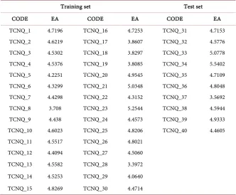
The descriptor considered in this work is electronic affinity (EA). This descrip-tor has been calculated according to Koopmans [45] approach: the electronic af-finity is the opposite of LUMO energy.

LUMO

EA= −E (25)

where LUMO is the Lowest Unoccupied Molecular Orbital. Table 2 reports the values of this descriptor for both the training set and the test set.

2.5. Submission of the Descriptor to the Selection Criterion 1

3. Resultats and Discussion

3.1. QSPR Model

The regression equation of the predictive QSPR (Quantitative Structure-Property Relationship) model of the first reduction potential dependent to electronic af-finity (EA) is given below:

1 _{2.5314 0.5708 EA}

theo

DOI: 10.4236/cc.2019.74009 133 Computational Chemistry

Table 2. Descriptor values expressed in eV, at B3LYP/6-31G(d,p) theory level.

Training set Test set

CODE EA CODE EA CODE EA

TCNQ_1 4.7196 TCNQ_16 4.7253 TCNQ_31 4.7153 TCNQ_2 4.6219 TCNQ_17 3.8607 TCNQ_32 4.5776 TCNQ_3 4.5302 TCNQ_18 3.8297 TCNQ_33 5.0778 TCNQ_4 4.5376 TCNQ_19 3.8085 TCNQ_34 5.5402 TCNQ_5 4.2251 TCNQ_20 4.9545 TCNQ_35 4.7109 TCNQ_6 4.3299 TCNQ_21 5.0348 TCNQ_36 4.8048 TCNQ_7 4.4298 TCNQ_22 4.3152 TCNQ_37 3.5692 TCNQ_8 3.708 TCNQ_23 5.2544 TCNQ_38 4.5944 TCNQ_9 4.438 TCNQ_24 4.4573 TCNQ_39 4.9333 TCNQ_10 4.6023 TCNQ_25 4.8206 TCNQ_40 4.4605 TCNQ_11 4.5517 TCNQ_26 4.8021

TCNQ_12 4.4094 TCNQ_27 4.5060 TCNQ_13 4.5582 TCNQ_28 3.3972 TCNQ_14 4.5253 TCNQ_29 4.0640 TCNQ_15 4.8269 TCNQ_30 4.4714

Table 3. Submission of the descriptor to the selection criterion 1.

Equation Coefficient of corrélation R Descriptors is selected if R≥0.50 ( )

1 EA

exp

E =f 0.9605 selected

2 2

adjusted

30; 0.9605; 0.9225; 0.9197; 0.0694;

333.3279; FIT 0.3469; -value 0.000; TSS 1.7407;

ESS 1.6058; 95%

n R R R s

F p

α

= = = = =

= = < =

= =

The positive sign of the coefficient of the EA in the regression equation of model shows that the first reduction potential increases with electronic affinity. There is therefore a direct correlation between the explanatory variable and the studied property. Examination of the above parameters shows that the correla-tion coefficient is very high (R=0.9605). This high value indicates that there is

a strong correlation between the first reduction potential and the selected de-scriptor. The determination coefficient 2

0.9225

R = shows that 92.25% of the

experimental variance of the first reduction potential is explained by the model's descriptor alone. In addition, the standard deviation (s=0.0694) tends towards

0, indicating a good fit and high reliability of the prediction. The p-value is less than 0.0001 so 1− =α 0.05 (5% risk). It is therefore clear that the regression

DOI: 10.4236/cc.2019.74009 134 Computational Chemistry to explain the studied property (first reduction potential). In addition, the expe-rimental variance is TSS = 1.7407 when the theoretical variance due to the model is ESS = 1.6058. It is important to note that this relationship of dependence be-tween the first reduction potential and electronic affinity has been corroborated by the work of Peter W. Kenny [46] who showed that the first reduction poten-tial is a function of LUMO energy. He developed a predictive QSPR model de-pendent only on LUMO energy calculated at HF/6-31G(d) theory level, from a series of sixteen analogous TCNQ molecules with statistical parameters (n=16;

2

0.969

R = ; F=436; s=0.04 V; α =95%). However, the internal and

ex-ternal validations of this model have not been studied. It is also important to note that a QSPR (Quantitative Structure-Property Relationship) model can be obtained in a hazardous way. Therefore, one must always make sure of its stabil-ity. To do this, both internal and external validations methods are performed.

3.2. Internal Validation of the Model

For internal validation, the Leave-One-Out (LOO) procedure and the property of the randomization test have been used.

 Leave-One-Out procedure

Table 4 indicates that the value of 2

LOO 0.9136

Q = . The model is therefore

excellent as seen 2

LOO 0.90

Q > [47]. In addition, 91.36 % of the molecules in the

training set have their redox potentials predicted by this model. With regard to the molecules of the training set, this model therefore has a high predictive power. This result shows that model is not very sensitive to this operation of set-ting apart a molecule and putset-ting it back into the training set (Leave-One-Out procedure). This justifies the stability of this model. For 2

(

)

LOO

m

r , its value is

greater than 0.50 when that of 2

(

)

LOO

m

r

∆ _{is less than 0.20. Consequently, for}

the prediction of the redox potential, the model is acceptable. Moreover, to en-sure that the model is not due to chance correlations, the Y-randomization test of the property has been realized. A circular permutation of the property has been made (29 iterations).

 Y-randomization test

The average values of the Y-randomization parameters are shown in Table 5. Table 5 shows that the average value of 2

r

R tends to 0 (R_r2=0.0600), show-ing that the equation of the regression line only determines 6.00% of the point distribution (redox potential). In addition, there is scatter around the regression line confirmed by a high standard deviation (sr =0.2415). The very low value of

the statistic Fr shows that the equation of the model obtained with the

rando-mized property is not significant. As for Todeschini’s parameter c 2

P

R , its value is

greater than 0.50 (c 2 _0.50

P

R > ). This confirms that the established model is not

due to chance correlations.

3.3. External Validation of the Model

DOI: 10.4236/cc.2019.74009 135 Computational Chemistry

Table 4. Statistical parameters of the LOO internal validation of the model.

n 2

LOO

Q 2( )

LOO

m

r ∆rm2(LOO) PRESS SDEP

30 0.9136 0.9136 0.0000 0.1504 0.0708

Table 5. Mean values of the randomization parameters.

Randomized parameter 2

r

R sr Fr

2

c P

R

Average value 0.0600 0.2415 1.9987 0.8920

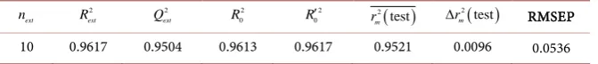
Table 6. Statistical parameters of the external validation of the model.

ext n 2 ext R 2 ext Q 2 0 R 2 0

R′ 2( )

test

m

r ∆rm2( )test RMSEP

10 0.9617 0.9504 0.9613 0.9617 0.9521 0.0096 0.0536

From the analysis of the data in Table 6, it appears that the model has a very

high predictive power because 2 _0.9504

ext

Q = . This shows that, 95.04% of

mole-cules of the test set have their redox potentials predicted by the model. Also, 96.17 % of the experimental variance of the first reduction potential is explained

by the descriptor model. For 2

( )

test

m

r , its value is greater than 0.50 while that of

( )

test

m

r

∆ _{is less than 0.2. Thus, this model is acceptable for the prediction of} the redox potential of the test set molecules. In addition, the five (05) criteria of external validation (Tropsha’s criteria) have been verified.

Verification of Tropsha’s criteria Criterion 1: 2

0.9617 0.70

ext

R = >

Criterion 2: 2 _{0.9504 0.60}

ext

Q = >

Criterion 3:

2 2

0

2 0.0004 0.1

ext

ext

R R

R

−

= < _and k=0.9905 avec 0.85< <k 1.15

Criterion 4:

2 2

0

2 0.0000 0.1

ext ext R R R ′ −

= < _and k′ =0.9797 avec

0.85<k′<1.15

Criterion 5: 2 2

0 0.0004 0.3

ext

R −R = <

At this level, we see that all five (05) Tropsha criteria are verified. As a result, the developed model is very efficient in predicting the first reduction potential of the series of studies molecules.

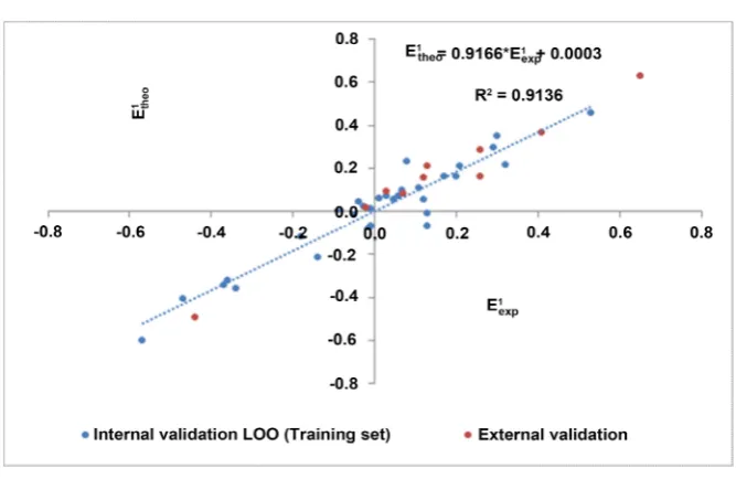
3.4. Correlation between the Predicted Values by the Model and

the Experimental Values

DOI: 10.4236/cc.2019.74009 136 Computational Chemistry

Figure 1. 1 1

exp

-theo

E E scatter diagram of the model.

Figure 2. Similarity between model-predicted values and experimental values.

3.5. Model Normality Tests

 Shapiro-Wilk’s test [48]

The data in Table 7 shows that the calculated p-value is greater than 1− =α 0.05

(5% threshold). Thus, the theoretical values of the first reduction potential ob-tained from the model follow a normal distribution law. This normal distribu-tion is confirmed by the distribudistribu-tion of the point cloud according to the first bi-sector in Figure 3.

 Durbin-Watson’s test [49]

The values in Table 8 show that the calculated p-value is greater than

1− =α 0.05 (5% threshold). It is therefore clear that the residues are not

DOI: 10.4236/cc.2019.74009 137 Computational Chemistry

Table 7. Values of the parameters of Shapiro-Wilk’s test.

Shapiro-Wilk’s parameter (W) p-value 1−α

0.9539 0.1036 0.05

Table 8. Values of the parameters of Durbin-Watson’s test.

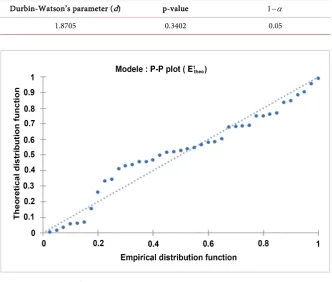
Durbin-Watson’s parameter (d) p-value 1−α

1.8705 0.3402 0.05

Figure 3. P-P plot ( 1

theo

E ) graph of the model.

Figure 4. Normalized residue =

(

)

theo

f E graph of the model.

3.6. Applicability Domain (AD) of the Model

DOI: 10.4236/cc.2019.74009 138 Computational Chemistry

Figure 5. Williams diagram of the model.

The examination of the Williams diagram shows that for training and test set, all observations have their standardized residuals between ±3 standard deviation units (±3σ) [50]. This justifies the absence of outliers. The choice “3 units of standard deviation” was made because our data follow a normal distribution law. Indeed, for leverage effect, a value of 3 is commonly used as a limit value for ac-cepting predictions because the points between ±3 standard deviation units cov-er on avcov-erage 99% of the data that follow a normal distribution law [51]. With regard to the levers of the training set, except for the observation TCNQ_28, all the others have their levers below the threshold value (h* _{= 0.2000). In the case of} the test set, it is observation TCNQ_34, which has its lever above the critical value. However, the value of a lever above the critical value does not always in-dicate an outlier for the developed model. Compounds of training set with levers above the threshold value with low residues stabilize the model and increase its accuracy. They are called “good influential points”. On the other hand, com-pounds with hii greater than the critical value h* with large residues are called “bad influencing points” [51]. As a result, our elaborate QSPR (Quantitative Structure-Property Relationship) model does not show any evidence of aberrant observation of molecules in either set. The molecule TCNQ_28 is a “good influ-ence point”. The results of the external validation showed that the model is suit-able for predicting future redox potentials of TCNQ of this same family belong-ing to its applicability domain.

4. Conclusion

The objective of this study was to develop a predictive QSPR (Quantitative Struc- ture-Property Relationship) model linking the first reduction potential from a series of tetracyanoquinodimethane molecules analogous to quantum descrip-tors from the conceptual density functional theory. A predictive QSPR model dependent to electronic affinity has been developed. The determination

coeffi-cient 2

0.9225

R = of this model shows that 92.25% of the experimental

DOI: 10.4236/cc.2019.74009 139 Computational Chemistry alone. The Fisher coefficient of this model is very high (F=333.3279)

indicat-ing that the regression equation is highly significant. The standard deviations (s=0.0694) are well below 0.50 indicating a good fit and high reliability of the

prediction. Regarding the parameters of the internal and external validations, they revealed that the model is validated and is assumed to predict efficiently the first reduction potential. The cross-validation coefficient 2

LOO 0.9136

Q =

indi-cates that 91.36% of molecules of the training set have their predicted first re-duction potential. Regarding the external validation coefficient, 2 _0.9504

ext

Q = ,

it shows that 95.04% of the test set molecules have their predicted first reduction potentials. Thus, to search for new tetracyanoquinodimethane (TCNQ) accep-tors of this same family with the desired first reduction potentials, one can play on electronic affinity.

Conflicts of Interest

The authors declare no conflicts of interest regarding the publication of this pa-per.

References

[1] Prasad, P.N. and Ulrich, D.R. (1988) Nonlinear Optical and Electroactive Polymers. Springer, Boston, 444 p.https://doi.org/10.1007/978-1-4613-0953-6

[2] Cuevas, J.C. and Scheer, E. (2010) Molecular Electronics: An Introduction to Theory and Experiment. World Scientific Publishing Co. Pte. Ltd., Singapore, 709 p.

https://doi.org/10.1142/7434

[3] Joran, A.D., et al. (1987) Effect of Exothermicity on Electron Transfer Rates in Photo-synthetic Molecular Models. Nature, 327, 508-511.

https://doi.org/10.1038/327508a0

[4] Shen, X.Y., et al. (2013) Effects of Substitution with Donor-Acceptor Groups on the Properties of Tetraphenylethene Trimer: Aggregation-Induced Emission, Solvatoch-romism, and Mechanochromism. The Journal of Physical Chemistry, 117, 7334-7347.

https://doi.org/10.1021/jp311360p

[5] Marcus, R.A. (1993) Electron Transfer Reactions in Chemistry. Theory and Expe-riment. Reviews of Modern Physics, 65, 599-610.

https://doi.org/10.1103/RevModPhys.65.599

[6] Klots, C.E., Compton, R.N. and Raaen, V.F. (1974) Electronic and Ionic Properties of Molecular TTF and TCNQ. The Journal of Chemical Physics,60, 1177-1178.

https://doi.org/10.1063/1.1681130

[7] Milián, B., Pou-Amérigo, R., Viruela, R. and Ortí, E. (2004) On the Electron Affinity of TCNQ. Chemical Physics Letters,391, 148-151.

https://doi.org/10.1016/j.cplett.2004.04.102

[8] Zhu, G.Z. and Wang, L.S. (2015) Communication: Vibrationally Resolved Photoe-lectron Spectroscopy of the Tetracyanoquinodimethane (TCNQ) Anion and Accurate Determination of the Electron Affinity of TCNQ. The Journal of Chemical Physics, 143, Article ID: 221102.https://doi.org/10.1063/1.4937761

[9] Pålsson, L.O., et al. (2003) Orientation and Solvatochromism of Dyes in Liquid Crystals. Molecular Crystals and Liquid Crystals, 402, 43-53.

DOI: 10.4236/cc.2019.74009 140 Computational Chemistry [10] Bloor, D., et al. (2001) Matrix Dependence of Light Emission from TCNQ Adducts.

Journal of Materials Chemistry,11, 3053-3062.https://doi.org/10.1039/b104992p [11] Cole, J.M., et al. (2002) Charge-Density Study of the Nonlinear Optical Precursor

DED-TCNQ at 20 K. Physical Review B, 65, Article ID: 125107.

https://doi.org/10.1103/PhysRevB.65.125107

[12] Bando, P., et al. (1994) Single-Component Donor-Acceptor Organic Semiconduc-tors Derived from TCNQ. The Journal of Organic Chemistry, 59, 4618-4629.

https://doi.org/10.1021/jo00095a042

[13] Arena, A., Patanè, S. and Saitta, G. (1988) Study of a New Organic Semiconductor Based on TCNQ and of Its Junction with Doped Silicon (TCNQ = 7, 7’8, 8’ Tetra-cyanoquinodimethane). Il Nuovo Cimento, 20, 907-913.

https://doi.org/10.1007/BF03185493

[14] Wheland, R.C. (1976) Correlation of Electrical Conductivity in Charge-Transfer Complexes with Redox Potentials, Steric Factors, and Heavy Atom Effects. Journal of the American Chemical Society, 98, 3926-3930.

https://doi.org/10.1021/ja00429a031

[15] Règlement (CE) n° 1907/2006 du Parlement Européen et du Conseil du 18 décem-bre 2006 concernant l’enregistrement, l’évaluation et l’autorisation des substances chimiques, ainsi que les restrictions applicables à ces substances (REACH), instituant une agence européenne des produits chimiques, modifiant la directive 1999/45/CE et abrogeant le règlement (CEE) n° 793/93 du Conseil et le règlement (CE) n° 1488/94 de la Commission ainsi que la directive 76/769/CEE du Conseil et les direc-tives 91/155/CEE, 93/67/CEE, 93/105/CE et 2000/21/CE de la Commission.

[16] Margossian, N. (2008) Le règlement REACH—La règlementationeuropéenne sur les produits chimiques. Dunod/L’Usine Nouvelle, Paris.

[17] Delaney, J.J. (1997) Synthesis of New Heterocyclic TCNQ Analogues. Doctorate of Philosophy, Dublin City University (School of Chemical Sciences), Dublin, 202 p. [18] Andersen, J.R. and Jorgensen, O. (1979) Organic Metals. Mono- and 2,5-Di-Substituted

7,7,8,8-Tetracyano-P-Quinodimethanes and Conductivities of Their Charge-Transfer Complexes. Royal Chemical Society, Journal of Perkin Transactions, 1, 3095-3098.

https://doi.org/10.1039/P19790003095

[19] Wheland, R.C. and Gillson, J.L. (1976) Synthesis of Electrically Conductive Organic Solids. Journal of the American Chemical Society, 98, 3916-3925.

https://doi.org/10.1021/ja00429a030

[20] Ferraris, J.P. and Saito, G. (1978) Organic Metals with Asymmetric Acceptors: The Monofluorotetracyanoquino-Dimethane Anion. Journal of the Chemical Society, Che- mical Communications, No. 22, 992-993.

https://doi.org/10.1039/C39780000992

[21] Saito, G. and Ferraris, J.P. (1979) Difluorotetracyanoquinodimethane: Electron Af-finity Cut-Off for “Metallic” Behaviour in a Tetrathiafulvalene Salt. Journal of the Chemical Society, Chemical Communications, No. 22, 1027-1029.

https://doi.org/10.1039/C39790001027

[22] Tsubata, Y., Suzuki, T., Yamashita, Y., Mukai, T. and Miyashi, T. (1992) Tetracya-noquinodimethanes Fused with 13, s-Thiadiazole and Pyrazine Units. Heterocycles, 33, 337-348.https://doi.org/10.3987/COM-91-S44

[23] Yamashita, Y. (1989) Novel Electron Acceptors and Donors Containing Fused-Hetero- cycles.Journal of Synthetic Organic Chemistry, 47, 1108-1117.

DOI: 10.4236/cc.2019.74009 141 Computational Chemistry [25] Frisch, M.J., Trucks, G.W., Schlegel, H.B., Scuseria, G.E., Robb, M.A., Cheeseman, J.R., Scalmani, G., Barone, V., Mennucci, B., Petersson, G.A., Nakatsuji, H., Carica-to, M., Li, X., Hratchian, H.P., Izmaylov, A.F., Bloino, J., Zheng, G., Sonnenberg, J.L., Hada, M., Ehara, M., Toyota, K., Fukuda, R., Hasegawa, J., Ishida, M., Nakaji-ma, T., Honda, Y., Kitao, O., Nakai, H., Vreven, T., Montgomery, J.A., Peralta, J.E., Ogliaro, F., Bearpark, M., Heyd, J.J., Brothers, E., Kudin, K.N., Staroverov, V.N., Kobayashi, R., Normand, J., Raghavachari, K., Rendell, A., Burant, J.C., Iyengar, S.S., Tomasi, J., Cossi, M., Rega, N., Millam, J.M., Klene, M., Knox, J.E., Cross, J.B., Bakken, V., Adamo, C., Jaramillo, J., Gomperts, R., Stratmann, R.E., Yazyev, O., Austin, A.J., Cammi, R., Pomelli, C., Ochterski, J.W., Martin, R.L., Morokuma, K., Zakrzewski, V.G., Voth, G.A., Salvador, P., Dannenberg, J.J., Dapprich, S., Daniels, A.D., Farkas, O., Foresman, J.B., Ortiz, J.V., Cioslowski, J. and Fox, D.J. (2009) Gaussian 09, Revision A.02. Gaussian, Inc., Wallingford.

[26] (2015) ACDLABS 10. Advanced Chemistry Development Inc., Toronto. [27] Microsoft® Excel® 2010.

[28] (2014) XLSTAT Version 2014.5.03, Copyright Addinsoft 1995-2014. [29] Minitab® 18.

[30] Vessereau, A. (1988) Méthodes statistiques en biologie et en agronomie. Lavoisier (Tec & Doc), Paris, 538 p.

[31] Chatterje, S. and Hadi, A.S. (2006) Regression Analysis by Example. 4th Edition, John Wiley & Son, Inc., Hoboken, 366 p.https://doi.org/10.1002/0470055464 [32] Siegel, A.F. (1997) Practical Business Statistics. IRWIN, 3rd Edition.

[33] Besse, P. (2003) Pratique de la modélisation statistique, Publications du laboratoire de statistique et Probabilité.

[34] Cook, R.D. and Weisberg, S. (1994) An Introduction to Regression Graphics. Wiley Series in Probability and Mathematical Statistics, Hoboken, 265 p.

https://doi.org/10.1002/9780470316863

[35] Kubinyi, H. (1994) Variable Selection in QSAR Studies. I. An Evolutionary Algo-rithm. Quantitative Structure-Activity Relationships, 13, 285-294.

https://doi.org/10.1002/qsar.19940130306

[36] Golbraikh, A. and Tropsha, A. (2002) Beware of q2! Journal of Molecular Graphics and Modelling, 20, 269-276.https://doi.org/10.1016/S1093-3263(01)00123-1 [37] Todeschini, R. (2010) Milano, Chemometrics and QSAR Research Group.

Univer-sity of Milano Bicocca, Milano.

[38] Roy, P.P., Paul, S., Mitra, I. and Roy, K. (2009) On Two Novel Parameters for Vali-dation of Predictive QSAR Models. Molecules, 14, 1660-1701.

https://doi.org/10.3390/molecules14051660

[39] Consonni, V., Ballabio, D. and Todeschini, R. (2010) Evaluation of Model Predictive Ability by External Validation Techniques. Journal of Chemometrics, 24, 194-201.

https://doi.org/10.1002/cem.1290

[40] Roy, K., Mitra, I., Kar, S., Ojha, P.K., Das, R.N. and Kabir, H. (2012) Comparative Studies on Some Metrics for External Validation of QSPR Models. Journal of Chemi-cal Information and Modeling, 52, 396-408.

https://doi.org/10.1021/ci200520g

[41] Tropsha, A., Gramatica, P. and Gombar, V.K. (2003) The Importance of Being Earnest: Validation Is the Absolute Essential for Successful Application and Inter-pretation of QSPR Models. QSAR & Combinatorial Science, 22, 69-77.

DOI: 10.4236/cc.2019.74009 142 Computational Chemistry [42] Ouattara, O. and Ziao, N. (2017) Quantum Chemistry Prediction of Molecular Li-pophilicity Using Semi-Empirical AM1 and Ab Initio HF/6-311++G Levels. Com-putational Chemistry, 5, 38-50.https://doi.org/10.4236/cc.2017.51004

[43] Gramatica, P. (2007) Principles of QSAR Models Validation: Internal & External. QSAR and Combinatorial Sciences, 26, 694-701.

https://doi.org/10.1002/qsar.200610151

[44] Netzeva, T.I., Worth, A.P., Aldenberg, T., Benigni, R., Cronin, M.T.D., Gramatica, P., Jaworska, J.S., Kahn, S., Klopman, G., Marchant, C.A., Myatt, G., Nikolo-va-Jeliazkova, N., Patlewicz, G.Y., Perkins, R., Roberts, D.W., Schultz, T.W., Stan-ton, D.T., Van De Sandt, J.J.M., Tong, W., Veith, G. and Yang, C. (2005) Current Status of Methods for Defining the Applicability Domain of (Quantitative) Struc-ture-Activity Relationships. Alternatives to Laboratory Animals, 33, 155-173.

https://doi.org/10.1177/026119290503300209

[45] Koopmans, T. (1933) Über die Zuordnung von Wellenfunktionen und Eigenwerten zu den Einzelnen Elektronen Eines Atoms. Physica, 1, 104-113.

https://doi.org/10.1016/S0031-8914(34)90011-2

[46] Kenny, P.W. (1995) Prediction of Planarity and Reduction Potential of Derivatives of Tetracyanoquinodimethane Using Ab Initio Molecular Orbital Theory. Journal of the Chemical Society, Perkin Transactions, 2, 907-909.

https://doi.org/10.1039/p29950000907

[47] Erikson, L., Jaworska, J., Worth, A., Cromin, M., McDowell, R.M. and Gramatica, P. (2003) Methods for Reliability, Uncertainty Assessment, and Applicability Evalua-tions of Regression Based and Classification QSPRs. Environmental Health Pers-pective, 111, 1361-1375.https://doi.org/10.1289/ehp.5758

[48] Shapiro, S.S. and Wilk, M.B. (1965) An Analysis of Variance Test for Normality (Complete Samples). Biometrika, 52, 591-611.

https://doi.org/10.1093/biomet/52.3-4.591

[49] Durbin, J. and Watson, G.S. (1951) Testing for Serial Correlation in Least Squares Regression, II. Biometrika, 38, 159-178.https://doi.org/10.1093/biomet/38.1-2.159 [50] Touhami, I., Mokrani, K. and Messadi, D. (2012) Modèles QSRR

hybridesalgorith-megénétique-régressionlinéaire multiple des indices de rétention de pyrazines en chromatographie gazeuse. Lebanese Science Journal, 13, 75-88.