Tests for an End-of-Sample Bubble in Financial
Time Series
Sam Astilla, David I. Harveyb, Stephen J. Leybourneb and A.M. Robert Taylora
a. Essex Business School, University of Essex.
b. Granger Centre for Time Series Econometrics and School of Economics, University of Nottingham.
September 28, 2016
Abstract
In this paper we examine the issue of detecting explosive behaviour in economic and …nancial time series when an explosive episode is both ongoing at the end of the sample, and of …nite length. We propose a testing strategy based on the sub-sampling method of Andrews (2003), in which a suitable test statistic is calculated on a …nite number of end-of-sample observations, with a critical value obtained using sub-sample test statistics calculated on the remaining observations. This approach also has the practical advantage that, by virtue of how the critical values are obtained, it can deliver tests which are robust to, among other things, conditional heteroskedasticity and serial correlation in the driving shocks. We also explore modi…cations of the raw statistics to account for unconditional heteroskedasticity using studentisation and a White-type correction. We evaluate the …nite sample size and power properties of our proposed procedures, and …nd that they o¤er promising levels of power, suggesting the possibility for earlier detection of end-of-sample bubble episodes compared to existing procedures.
Keywords: Rational bubble; Explosive autoregression; Right-tailed unit root testing:
Sub-sampling.
JEL Classi…cation: C22; C12; G14.
We are grateful to the Guest Editors, Peter Phillips and Aman Ullah, and two anonymous referees for their
helpful and constructive comments on earlier versions of this paper. Address correspondence to: Robert Taylor,
1
Introduction
The e¢ cacy of unit root tests for detecting explosive rational asset price bubbles is well
docu-mented. In the seminal paper on the presence of explosive rational asset price bubbles in stock
prices by Diba and Grossman (1988), the authors note that if the bubble component of a stock
price series follows an explosive autoregressive process, the explosive behaviour caused by the
bubble component is still manifest in the …rst di¤erence of the series. This is due to the fact
that an explosive autoregressive process cannot be di¤erenced to stationarity. As such, if a
series is found to be non-stationary in levels, but stationary in …rst di¤erences, then the series
is not subject to explosive behaviour. Based on this, Diba and Grossman (1988) propose testing
the null hypothesis of no explosive behaviour by applying standard left-tailed regression-based
unit root tests to a series in both levels and …rst di¤erences. Recent research on the detection
of asset price bubbles, however, has concentrated on applying right-tailed Dickey-Fuller [DF]
tests to the levels of a series. The earliest contribution to this approach in the literature was
made by Phillips, Wu and Yu (2011) [PWY], who propose a test procedure for detecting
ex-plosive rational bubbles in stock markets based on the supremum of a set of forward recursive
right-tailed DF test statistics applied to both the price and dividend series in levels. If explosive
behaviour is found in the price series, but not in the dividend series, they conclude that the
stock price is subject to an explosive rational bubble. PWY apply their test procedure to the
NASDAQ composite stock price and dividend index for the period from February 1973 –June
2005 and identify the emergence of the dot-com bubble in the middle of 1995.
Due to the simplicity of the PWY test procedure, and its favourable power properties, this
test procedure has been utilised extensively in the both the …nance and econometrics literature
to detect bubbles in a number of …nancial series. Gilbert (2010) applies the PWY test procedure
to commodities futures prices for the years 2000-2009 and …nds evidence of explosive behaviour
in the nickel, copper and crude oil series. Homm and Breitung (2012) apply both the PWY
test and a Chow-type test to various series including stock prices, commodity prices and house
prices, …nding evidence of bubbles in a number of the series examined. Bettendorf and Chen
(2103) apply the PWY test procedure to the sterling-US dollar exchange rate and …nd evidence
of explosive behaviour in the exchange rate driven by explosive behaviour in the price index for
traded goods. In a subsequent paper aimed at dealing with the issue that more than one asset
price bubble could potentially be present within a given sample of data, Phillips, Shi and Yu
(2015) [PSY] propose a test for at least one bubble based on a supremum of right-tailed DF
statistics computed over all possible start and end dates (subject to a minimum sample size).
If a rejection is obtained by this test, PSY propose a dating procedure to identify the timing
of the bubble episodes, which uses sequential application of a sequence of backward recursive
right-tailed DF statistics.
Based on the aforementioned evidence for the presence of explosive asset price bubbles,
imperative that bubbles are detected as early as possible. Arguably, the most useful application
of tests for asset price bubbles to policy makers is detecting an ongoing asset price bubble as
soon as possible. Thus, our focus in this paper is on testing for an explosive asset price bubble
of …nite length that is ongoing at the end of the sample. Whilst most tests proposed in the
literature concentrate on detecting and dating past asset price bubbles, the backward recursive
approach of PSY is particularly well-suited to detect an end-of-sample bubble. A potential
drawback of the PSY approach to bubble detection, however, is that for its asymptotic validity,
it assumes that the length of the bubble regime is some non-vanishing fraction of the total
sample size. In the context of detecting end-of-sample bubbles quickly, a more appropriate
assumption might be one of a …nite length end-of-sample bubble regime, because possibly only
a few bubble observations might have been observed at the time when the tests are executed.
The approach we consider in this paper is based on the end-of-sample instability testing
approach developed by Andrews (2003) and Andrews and Kim (2006). This involves calculating
a test statistic based on a …nite sized window of end-of-sample observations, and comparing
this with critical values obtained by sub-sampling across the remaining earlier observations.
This approach, by design, delivers tests which are robust to serial correlation and conditional
heteroskedasticity in the driving shocks, without the need for any correction (parametric or
non-parametric) to the test statistics. In this paper we propose such Andrews-type tests, adapted
to the case of testing the null of no end-of-sample bubble against the bubble alternative. The
statistics we consider for this Andrews-type approach take the form of: (i) a right-tailed DF
statistic (notice that because of the robustness to serial correlation mentioned above, no lags are
needed in the DF test regression), and (ii) implementations of the Andrews and Kim (2006)-type
statistics that are motivated by a …rst order Taylor series expansion of the …rst di¤erences of
an explosive autoregressive process. We …nd that all these procedures o¤er decent …nite sample
size control, and the Andrews-Kim-type variants in particular o¤er promising levels of power,
suggesting the possibility for earlier detection of end-of-sample bubble episodes compared to
extant procedures.
When testing for the possibility of changing autoregressive dynamics in …nancial series, it
can also be important to recognise that the underlying innovation process may be susceptible to
changes in unconditional variance. To this end, we also consider variants of the above procedures
that are robust to heteroskedasticity. A studentisation of the Andrews and Kim (2006)-type
statistics automatically delivers tests which are robust to breaks in the unconditional volatility of
the driving shocks occurring before the end-of-sample window of observations used to compute
the statistics. To achieve robustness to a wider class of heteroskedastic processes, including
volatility changes that occur during the end-of-sample window, we propose a further correction
to the statistics based on a White-type heteroskedasticity adjustment. Following Harvey et al. (2016) [HLST] who proposed wild bootstrap versions of the PWY test, we also consider a wild bootstrap variant of the backward recursive approach of PSY in order to also render this
The remainder of the paper is organised as follows. In section 2 we outline the model and
present our proposed test procedures. The …nite sample size and power properties of the tests
are examined in section 3 using Monte Carlo simulations, where comparisons are made with
the PSY approach. In section 4 we consider extensions to the proposed tests, and also to the
PSY approach, that are robust to heteroskedasticity, and assess the …nite sample and power
properties of the di¤erent procedures. Section 5 presents an application to the same S&P500
price-dividend ratio data studied by PSY, and section 6 concludes.
2
The Model and Tests for an End-of-Sample Bubble
Consider a time series processfytggenerated according to the following data-generating process
[DGP]
yt = +ut; t= 1; :::; T+m (1)
ut = (
ut 1+"t; t= 1; :::; T
ut 1+"t; t=T + 1; :::; T +m
(2)
where u0 = Op(1) and where, following Andrews (2003) and Andrews and Kim (2006), we
assume the innovation processf"tg is mean zero, stationary and ergodic. The series yt follows
a unit root process for the …rst T observations and is then subject to (potential) explosive
behaviour for the …nal m observations (wherem is considered to be small relative to T). The
null hypothesis (H0) of no explosive behaviour corresponds to = 1in (2), so that ytremains
unit root throughout the entire sample of T+m observations, while the alternative (H1) of an
end-of-sample explosive regime occurs when >1 in (2).
Standard Dickey-Fuller-type approaches to testingH0againstH1have been developed (see,
among others, PWY, Homm and Breitung, 2012, and PSY), and rely on large sample theory to
establish properties of their test procedures, implicitly treating the length of the bubble regime
to be of order T. Given that our focus is on developing tests to detect end-of-sample bubble
behaviour inyt when there are only a few observations from the bubble regime in the sample,
an alternative approach to consider is that of the end-of-sample instability tests that follow the
work of Andrews (2003) and Andrews and Kim (2006), where the asymptotics rely onT ! 1
while, importantly, m is allowed to remain …nite. Initially treating m as known, the general
Andrews-type approach involves calculating a test statistic based on a …nite length window ofm
end-of-sample observations, and comparing this with critical values obtained by sub-sampling
using the …rst T observations. Speci…cally, T m+ 1 analogous test statistics are computed,
each using a rolling window of m observations, from t = 1; :::; mto t = T m+ 1; :::; T; the
-level critical value is then equal to the1 empirical quantile of theseT m+ 1sub-sample
statistics. In this paper we consider a number of suitably designed tests within this
Andrews-type framework, where the intention is to distinguish between H0 : = 1and H1 : >1 by
obtained from this same statistic applied to theT m+ 1prior sub-samples.
A natural candidate statistic to use in the Andrews-type approach is the Dickey-Fuller
t-ratio (DFm) associated with the OLS estimator of in the regression
yt= + yt 1+"t; t=j+ 1; :::; j+m
de…ned for the sub-samples j 2 [1; :::; T m] (for critical value calculation) and j = T (for
the test statistic), where a rejection of H0 in favour of H1 is signalled by an upper-tail
rejec-tion. Notice that lagged di¤erence augmentation is not required because any dependence in
"t is common to all sub-samples. Under our assumptions, the Andrews-type approach applied
to DFm will result in a correctly sized test under H0 for large T. A potential problem for
this implementation of the Andrews-type approach is that the estimator of the autoregressive
parameter is likely to be inaccurate for the small values we envisage using for m, which may
have a detrimental e¤ect on power.
A simple alternative statistic to employ in the Andrews-type framework can be motivated
by considering the properties of the …rst di¤erences of yt. Under H0, it is clear that yt="t
throughout the full sample period, while under H1, yt="t up to timet=T, at which point
the bubble regime commences and yt = ( 1)ut 1+"t. De…ning the explosive o¤set >0
as := 1, we can write, for t=T+ 1; :::; T+m,
ut = (1 + )t TuT + t TX1
j=0
(1 + )j"t j
yt = ut
= (1 + )t T 1uT + t TX1
j=0
(1 + )j "t j: (3)
Notice that the stochastic behaviour of yt is dominated by the …rst term on the right hand
side of (3), with, for …nitem, (1 + )t T 1u
T =Op(T1=2)and Pjt T=0 1(1 + )j "t j =Op(1).
Next consider approximating (1 + )t T 1 using a …rst order Taylor series expansion around
= 0. We …nd
(1 + )t T 1 1 + (t T 1)
giving the approximation
yt= (1 )uT + 2uT(t T) +et (4) where et contains the higher order terms in the Taylor series expansion and the Op(1) term
from (3).
Using the approximation in (4), an obvious candidate statistic for an Andrews-type
instabil-ity test would be theF-statistic for joint signi…cance of the estimated coe¢ cients in a regression
of yt on uT and uT(t T), which is identical to calculating the F-statistic in a regression
does not take account of the fact that the form of explosive behaviour we are trying to detect
imposes positivity constraints on both the constant and linear trend terms in (4). A natural
one-sided possibility would be to focus on just the trend term, and simply test for an upward
trend in a regression of yt on a constant and linear trend using at-statistic. The drawback
of this approach is that it involves estimating the constant term in all of the rolling sub-sample
regressions from which the critical value is obtained (as well as the end-of-sample regression).
This constitutes an ine¢ cient approach to testing because it does not make use of the fact that
the rolling sub-samples up to timeT contain a zero intercept in population terms.
An alternative is instead to simply test for an upward trend in a regression of yt on
a linear trend alone using a standard t-statistic. This is correctly speci…ed for the rolling
sub-sample statistics (relevant for the critical value); the end-of-sample statistic is then based
on an under-speci…ed model, but will retain power against H1 nonetheless, and unreported
simulations con…rm that this restricted testing approach yields higher power than either the
F-statistic approach or the t-statistic approach that …ts a constant. The restricted regression
t-statistic in question is a studentised version of the trend coe¢ cient estimator
Pj+m
t=j+1(t j) yt
Pj+m
t=j+1(t j)2
de…ned for the sub-samplet=j+1; :::; j+m, withj2[1; :::; T m](for critical value calculation)
and j =T (for the test statistic). In fact, given the nature of the Andrews-type methodology,
we can simply consider the numerator
Sm := jX+m t=j+1
(t j) yt
because the denominator is numerically identical across j, and neither is a studentisation
re-quired under the assumption that "t is stationary and ergodic. Under our assumptions, the
Andrews-type approach applied toSm will result in a correctly sized test under H0 for largeT.
It is interesting to note the relation ofSm to theR statistic of Andrews and Kim (2006) for
testing an end-of-sample change from I(0) to I(1) behaviour. In the present context, ytis I(0)
up to time T, and, given that an explosive autoregressive process retains explosive behaviour
when …rst di¤erenced, it would be expected that a test for a change to I(1) behaviour in yt
will also reject in the presence of a change to explosivity. The Andrews-KimR statistic in this
context would be
Rm:= jX+m t=j+1
jX+m s=t
ys
!2
:
Note that our statisticSm can equivalently be expressed as
Sm = jX+m t=j+1
jX+m s=t
ys (5)
An attractive feature of the Andrews-type approach is that the asymptotic (inT) size ofS
(andR) will be una¤ected by the presence of a …nite number of bubbles, each of …nite length,
occurring earlier in the sample period. This arises because the yt from these bubble regimes
a¤ect only an asymptotically negligible number of the sub-sample statistics used for computing
the critical value.
In practice, the true value of the putative bubble regime length m is of course unknown.
In the remainder of the paper we use m0 to denote the sub-sample window width used when
construction the tests, denoting the procedures hereafter by Sm0, Rm0 and DFm0, retaining m
as the DGP parameter in (1)-(2).
3
Finite Sample Simulations
In this section we perform a set of Monte Carlo simulation exercises to examine the …nite
sample (empirical) size and power properties of the end-of-sample Sm0, Rm0 and DFm0 tests
proposed in the previous section. Because in practice the true value of m (the length of the
end-of-sample bubble period) will be unknown, we will consider the properties of the tests with
di¤erent window width settings,m0.
The performance of these tests is assessed in relation to a recursive Dickey-Fuller-based
approach following the work of PWY and PSY. Of the procedures proposed by PWY and PSY,
the most suitable for testing for the presence of a bubble that occurs at the end of the sample
period is an implementation of theBSADF test of PSY. Speci…cally, we consider the statistic
BSADF := sup r2[0;1 r0]
ADFr1
where ADFr1 denotes the standard augmented Dickey-Fuller statistic based on …tting the fol-lowing regression
yt= + yt 1+
k
X
i=1
k yt k+ errort
over the sub-sample period t = brT c+ 1; :::; T (where b:c denotes the integer part of its
argument), with T the sample size (i.e. T := T +m). The BSADF statistic is therefore
a supremum of a sequence of backward recursive unit root statistics running to the end of
the sample period. The minimum sub-sample length is given by br0T c, with r0 chosen to
ensure that the sub-samples exceed an appropriate minimum length; we follow PSY and set
r0 = 0:01 + 1:8=
p
T . PSY recommend using a small …xed lag length in the Dickey-Fuller
regressions, so in the simulations that follow the BSADF test statistic is calculated with
k = 1. The limiting null distribution of the BSADF statistic is obtained from the result in
equation (5) of PSY, on …xingr2 = 1. We employ asymptotic critical values for this test, and
we obtained these by simulating the limiting null distribution.
All Monte Carlo simulations that follow were conducted in Gauss 9.0. The size simulations
all tests being performed at the nominal 0.05-level. We generate data according to the DGP
(1)-(2), setting = 0 without loss of generality, and with an initial valueu0 = 100, chosen such
that under the alternative hypothesis, the bubbles generated are generally upwardly explosive (note that the tests are invariant to u0 under the null).
3.1 Empirical Size
To examine the size of the test procedures discussed in this paper, we set = 1, and let "t
be generated according to the moving average process "t = vt+ vt 1 with vt IIDN(0;1)
for =f0; 0:3; 0:5g. Table 1 reports the empirical size of the test procedures for the total
sample sizes T :=T +m =f100;200g, where theSm0, Rm0 and DFm0 tests are implemented
using m0 = 5 and m0 = 10.
The overall picture from Table 1 is that all procedures control size fairly well, particularly
for the larger sample size, and with the exception of BSADF, the tests are largely una¤ected
by the presence of serially correlated innovations. Concentrating on the IID case = 0, we
see that for the smaller sample size ofT = 100 the newly proposedSm0,Rm0 and DFm0 tests
exhibit some modest oversize; the size of these tests is also increasing in the window width,
m0, used in their construction. The BSADF test also exhibits mild oversize in this scenario,
with maximum size similar to S5,R5 and somewhat lower thanS10, R10. As we increase the
sample size the degree of oversize exhibited by the tests is generally decreasing. The reduction
in oversize for Sm0, Rm0 and DFm0 is due to the fact that, as the sample size increases, we
are able to calculate more sub-sample test statistics, allowing more accurate calculations of the
critical values of the tests. For non-zero values of we see a distinction between the BSADF
test and our proposed Sm0,Rm0 and DFm0 tests. While the latter three are little a¤ected by
the value of for any sample size, theBSADF test can su¤er from undersize for the negative
values of considered. The relative robustness of the Sm0, Rm0 and DFm0 tests to moving
average components is explained by the fact that the same serial correlation properties present
in observations used by the end-of-sample statistic are also present in all of the sub-sample
statistics used for critical value computation, thereby rendering the size of the test relatively
una¤ected.
Given that the undersize observed for BSADF could be attributable to the fact that k
in the Dickey-Fuller regressions is …xed at k = 1 rather than being data-dependent, we also
investigated the properties of BSADF where k is chosen according to the Bayes Information
Criterion (BIC). Table 1 also reports results for this variant, which we denote by BSADFB,
and where the maximum value of k is set to 6. We …nd that the undersize is indeed generally
removed, but at the expense of substantial oversize, particularly forT = 100and also for >0
for the larger sample sizes. As a result, we do not consider theBSADFB procedure further in
3.2 Empirical Power
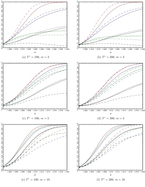
We now examine the power of the tests to detect an end-of-sample bubble. To do so, we generate
"t IIDN(0;1)innovations, and consider bubble lengths of m=f2;5;10g in sample sizes of
T =f100;200g. Figure 1 reports power curves across 2 [1; max] using a grid of 50 steps, with max = 1:05 for m = 2, and max = 1:02 for m = 5 and 10, respectively (re‡ecting the fact that, for a given value of , a bubble of longer duration is easier to detect).
For the shortest bubble length, m= 2, there is a fairly clear ranking of the tests in terms
of power, with the best overall performance given by the Sm0 tests, followed by the Rm0 tests,
with the results qualitatively similar across T = 100 and T = 200. The DFm0 tests exhibit
substantially lower power, and theBSADF test has the poorest power performance of all. It
is clear, then, that the Sm0 and Rm0 tests are well suited to detect end-of-sample bubbles of
very short duration, unlike theDFm0 andBSADF tests. It is also interesting to note that the
choice of the end of sample window width, m0, used in the Sm0 and Rm0 tests has an impact
on their respective power levels, with the shorter window settings (i.e. S5 and R5) delivering
relatively higher power for this short duration end-of-sample bubble than the longer window
widths (i.e. S10 and R10). This ranking is reversed for the DFm0 tests, whereDF5 has lower
power than DF10.
Moving to the case ofm= 5, we observe a broadly similar power ranking among the tests.
In particular, theSm0 tests continue to display the best overall power pro…les, with both window
width variantsS5 andS10 now emerging as unambiguously the most powerful procedures. The
power of the Rm0 tests again lie between the power curves for theSm0 and BSADF tests, but
interestingly, the power of theDFm0 tests is now very sensitive to the choice of m0, with DF5
displaying very low power levels, below that ofBSADF.
For the case of m = 10, all the DFm0 tests have poor power performance, while BSADF
now has a more competitive power pro…le for this bubble of longer duration. The power of the
S5 andR5 tests is lower for this case where the bubble duration is considerably longer than the
window width used in the tests; this arises because bubble observations are now being included
in the sample period from which the critical values are derived. However, the S10 test retains
its position as the best performing test.
From a real-time monitoring perspective, it is interesting to investigate how quickly a bubble
is likely to be detected by the di¤erent procedures. One way of measuring this speed of detection
is to examine the powers of the tests when the sample contains just a single bubble observation
at the end, then when the last two observations correspond to the bubble regime, then the last
three, and so on. Other things being equal, a good test for real-time monitoring purposes will
be one that has high power for a low number of bubble observations, so that in practice the null
would be expected to be rejected in favour of a bubble relatively early into the bubble regime.
We now consider such power comparisons, restricting our attention to the best-performing
a single end-of-sample bubble of length m = 20. We initially apply the tests to the simulated
series using only the observations t = 1; :::;160, thereby evaluating the rejection frequencies
of the tests as if we were at the point in time 160. We then repeat the simulation exercise
using the observations t = 1; :::;161, again calculating the rejection frequencies of the tests
(now associated with time period 161), and continue in this manner until we are simulating
the rejection frequencies based on the full sample t = 1; :::;200. Of course, for the simulation
experiments up to and including time period180, no bubble is present in the data so we expect
to see rejection frequencies close to the nominal size for these cases. After this point, a bubble
is present of increasing duration, and we can evaluate the powers of the tests to detect it, giving
an indication of the relative performance of the procedures to provide an early warning of a
bubble in an evolving real-time situation.
Denoting the end-date of the sample to which the tests are applied by E, Figure 2 reports
the rejection frequencies of theSm0 and BSADF tests forE =f160;161; :::;200g for = 1:01
and = 1:02.1 We observe that the rejection frequencies for all the tests are approximately
equal to their nominal size up to E= 180, after which time the bubble enters the samples and
the rejection frequencies begin to rise. It can be seen that the powers reinforce the results from
our earlier power simulations, with theSm0 test most likely to reject early into the bubble than
BSADF. As we move further into the bubble, the rejection frequency of some of theSm0 tests
begins to plateau or decrease; this feature arises because whenE >180 +m0, the critical values
start to increase due to contamination by bubble observations. TheBSADF test is not subject
to these power decreases due to its construction, and power continues to rise with increasing
numbers of bubble observations. However, the results demonstrate that it is theSm0 procedure
that is particularly well-suited to early detection of an end-of-sample bubble.2
4
Accounting for Heteroskedasticity
The tests considered thus far implicitly assume that the unconditional variance of the innovation
process f"tg is constant throughout the sample period. However, when dealing with …nancial
time series, it is important to recognise that the underlying innovations may be susceptible to
1
Note that theBSADF results depend on but do not of course change across the settings form0; the results
are simply repeated for ease of comparison. Figure 2 also reports results for tests that will be introduced and
discussed later in the paper. 2
In a companion discussion paper version of this paper (Astillet al., 2016), we also considered DGPs where
a bubble abruptly collapses after a number of periods, and also examined the impact of a previously collapsed
bubble on the power of the tests to detect an end-of-sample bubble. Overall, we …nd similar power patterns to
those in Figure 2, apart from when a previously collapsed bubble is relatively close to the end-of-sample bubble.
In this latter case, theSm0 tests recover their properties from the collapse of the …rst bubble much more rapidly
than theBSADF test, which has relatively poor power to detect the second bubble. Of course, a prior bubble
of long duration can adversely a¤ect the powers of theSm0 tests, since a large proportion of sub-sample statistics
used for computing the critical values are a¤ected by the earlier bubble, hence caution should be exercised if a
variance changes. To this end, we now consider variants of the better-performing Sm0 tests
that account for unconditional heteroskedasticity (note that conditional heteroskedasticity is
already permitted under the conditions on"t; see Andrews, 2003).
A …rst step in this direction would be to consider a simple studentised version ofSm0, taking
the form
Sm0 :=
Sm0
qPj+m0 t=j+1( yt)
2: (6)
Such a modi…cation imbues theSm0 tests with robustness to a …nite number of volatility shifts
that occur over the period t = 1; :::; T m0. This arises because, for all sub-samples which
do not contain a variance break, the statistics are correctly studentised, while only a …nite
number of sub-sample statistics will have a studentisation that is contaminated by the variance
change. Given that only an asymptotically negligible number of the sub-sample statistics used
for computing the critical value are a¤ected, Sm0 will be asymptotically correctly size. While Sm0 would not deliver size control if a volatility shift occurred in the …nal m0 observations of
the series, in some circumstances it may be deemed that the greater concern is robustness to
volatility shifts that arise over the much longer sample period used to obtain the critical values.
A further modi…cation that would produce a test robust to unconditional heteroskedasticity
of more general form across the full sample period (including the …nal m0 observations) is to
adopt a White-type correction in the studentisation, i.e.:
Smw0 :=
Sm0
qPj+m0
t=j+1f(t j) ytg2
: (7)
In what follows we assess the relative size and power performance of Sm0 and Smw0, under both
homoskedastic and heteroskedastic DGPs, and also consider their properties in relation to the
unmodi…edSm0 tests.
In a recent paper, HLST developed wild bootstrap variants of the PWY test that deliver
asymptotic robustness to non-stationary volatility. In the current setting, it is natural to
consider a similar wild bootstrap approach applied to the BSADF statistic outlined above,
which will also serve as a useful comparator for the Sm0 and Smw0 tests. HLST propose two
bootstrap algorithms, one based on the wild bootstrap applied to the …rst di¤erences of the
series, the other based on the wild bootstrap applied to residuals from a …tted model, which
makes use of the BIC-based approach of Harvey, Leybourne and Sollis (2016). We also consider
the equivalent two wild bootstrap methods here, although in the latter case, because we are
purely interested in modelling a putative bubble that occurs at the end of the sample, we restrict
attention to Model 1 of that paper in the model …tting stage, thereby …tting a unit root to
bubble model with the change-point date identi…ed by minimising the sum of squares residuals.3
Asymptotic results similar to those of HLST would apply to such bootstrap tests, ensuring the
3
The HLST dating methodology only identi…es valid bubble dates where the end of bubble date (denotedyT
here) exceeds the start of bubble date (denotedyT here). In cases where this is not satis…ed for anyT, we revert
asymptotic validity of these procedures under heteroskedasticity of the form considered here.
In the sequel, we denote the …rst di¤erence-based wild bootstrap approach by BSADF1
b, and
the model-based variant by BSADFb2.
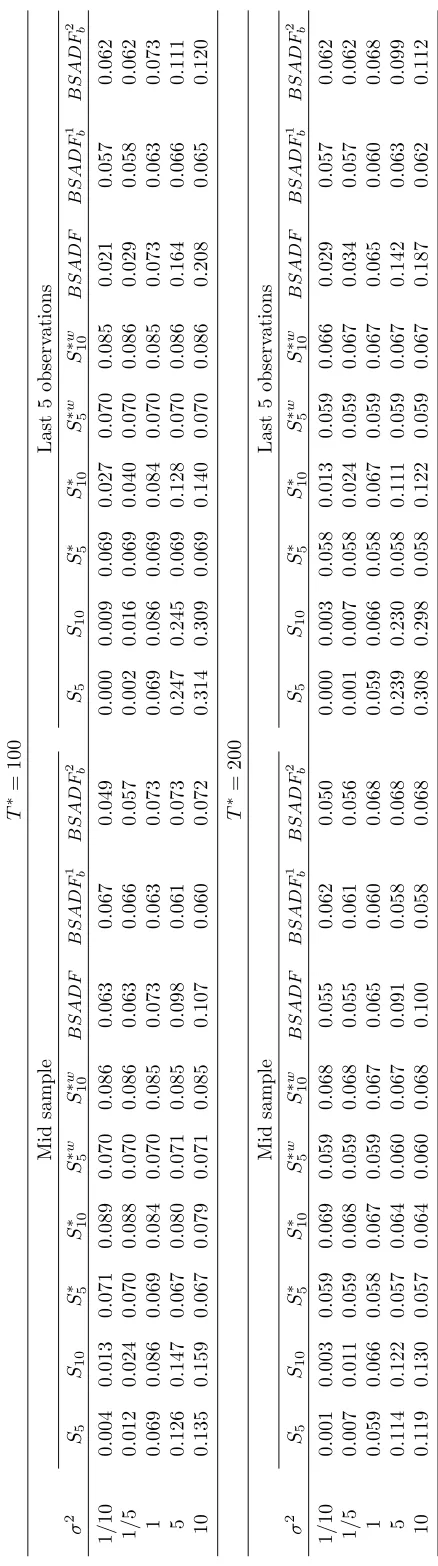
We now evaluate the …nite sample size and power of the heteroskedasticity-adjusted tests
using a similar set of Monte Carlo simulations to those of the previous section. Table 2 reports
the sizes of Sm0, Smw0, BSADFb1 and BSADFb2, along with the original Sm0 and BSADF
tests for comparison. Here, we introduce a single shift in the variance of the innovations,
with "t IIDN(0;1) for t = 1; :::; T and "t IIDN(0; 2) for t = T + 1; :::; T , for 2 =
f1=10;1=5;1;5;10g. We consider two cases: (i) T = T =2, allowing for a mid sample shift, and (ii) T = T 5, where the shift occurs …ve observations from the end of the sample,
commensurate with our focus on changes occurring late in the sample period. First, in the
homoskedastic case ( 2 = 1), we …nd that the S5,S5w and S10,S10w tests display very similar sizes to their uncorrected counterpartsS5 andS10, respectively. Similarly, the size ofBSADFb2
is similar to that ofBSADF, with the size ofBSADF1
b a little lower.
When the innovation variance changes, the impact on the tests is dependent on both the
timing and the direction of the change. The unadjusted testsS5,S10andBSADF lack
robust-ness to 2, and, relative to the homoskedastic case, size decreases when there is a downward variance shift, and size increases when the shift is upwards. The extent of the size distortions
is relatively modest in the case of a mid sample variance change, but is more exaggerated when
the change occurs late. Indeed, quite large oversize is seen in all these tests when a late upward
change arises. For the S5 and S10, as would be expected, size robustness is seen when the volatility change occurs mid sample, although when the volatility change is only present in the
last …ve observations, theSm0 approach does not generally deliver robustness. This is seen in the
size distortions manifest in theS10test, with undersize associated with an increase in variance, and oversize with a decrease in variance. Note that here, S5 is numerically invariant to 2 as the window width coincides with the number of observations in the …nal variance regime for this
particular case. TheSmw0 tests achieve good size control across 2 when T = 200,
demonstrat-ing the robustness of this approach to heteroskedasticity. When T = 100, some upward size
distortions are present, but these are modest in nature compared to the unadjusted tests. The
asymptotically heteroskedasticity-robust BSADFb1 and BSADFb2 tests improve …nite sample size relative toBSADF, although theBSADFb2 variant can still have size in excess of0:10for late upward volatility shifts, even whenT = 200.
Figure 3 reports …nite sample power results for Sm0,Smw0,BSADFb1 and BSADFb2 for the
same homoskedastic DGPs as were considered in Figure 1. The originalSm0 andBSADF power
curves are also super-imposed for comparison purposes. Consider …rstm= 2where the bubble
begins very close to the sample end. It is evident that the heteroskedasticity corrections applied
to Sm0 and Smw0 have a cost in terms of power, with the power ranking being, for a given m0, Sm0 followed bySm0 and then Smw0. As with theSm0 tests, S5 outperforms S10 here, although
of power to BSADF, as might be expected given the results of HLST who show that this wild
bootstrap approach involves no loss in (size-adjusted) power. It is noticeable that BSADF1
b
does not achieve the same power asBSADF, in contrast to HLST’s …ndings for this test when
applied to bubbles of longer duration. On comparing the Smw0 and BSADFb2 tests, Smw0 o¤ers
higher power for the smaller values of , while the ranking is reversed for larger , suggesting
a possible role forBSADFb2 in the early detection of large bubbles. Turning to m= 5, we see that Sm0 and Smw0 have levels of power closer to each other, and also closer to the uncorrected
Sm0 tests. Here, theSm0 andSmw0 tests have superior power toBSADFb2 (andBSADFb1) across
for both values of m0. Form= 10, theS10w becomes the best performing of all the corrected tests, dominatingS10 and BSADFb2, as well as S5 and S5w. On the basis of these results, our recommendation would be for the S10 test in the absence of heteroskedasticity concerns, and
theS10w variant if full robustness to heteroskedasticity is desired.
The rejection frequency simulations across sample end-dates reported in Figure 2 also
con-tain results for theSm0,Smw0,BSADFb1 andBSADFb2 tests. In line with the results of Figure
3, we observe that the Sm0 and Smw0 follow the same broad rejection patterns asSm0, but with
reduced power levels. It can be seen that across all the …gures,Sm0 is more likely to reject early
into the bubble regime compared with Smw0, but then the Sm0 tests achieve a greater rejection
frequency when further into the bubble. TheBSADFb2 test displays a similar rejection pattern toBSADF (again in line with Figure 3), with the BSADF1
b powers somewhat lower. As was
the case withBSADF,BSADFb1 and BSADFb2 have power that always rises with increasing numbers of bubble observations, while theSm0 andSmw0 powers eventually plateau and decrease.
As before, however, the Andrews-based approaches deliver greater early rejection frequencies
than theBSADF approach and its bootstrap variants.
Finally, in Figure 4 we consider powers when heteroskedasticity is present in the innovations.
We restrict attention to T = 200 and m = 5, and simulate the powers of the Sm0, Smw0, BSADF1
b andBSADFb2 tests for four cases, covering both a mid sample increase and decrease
in volatility ( 2 = 1=5 and 2 = 5), and volatility shifts of the same magnitude that occur in the last …ve observations. Consider …rst the results for the mid sample volatility shifts. Here,
all tests are asymptotically robust to the heteroskedasticity, as is re‡ected in the = 1 power
curve intercepts. Compared to the corresponding DGP without any variance shift (i.e. Figure
3(d)), the powers of the tests are increased for 2= 1=5and decreased for 2 = 5. However, the relative rankings of the procedures are broadly una¤ected by the presence of heteroskedasticity,
with the most noticeable feature being the dominance of Sm0 and Smw0 over BSADFb1 and BSADFb2. When the variance change applies only to the last …ve observations,S10is no longer robust, and is subject to undersize when 2 = 1=5 and oversize when 2= 5. For the volatility decrease, the Smw0 tests substantially outperform BSADFb1 and BSADFb2, while the ranking
is less clear with respect to BSADFb2 when the volatility increases, partly because BSADFb2
displays some …nite sample oversize in this case. Overall, our recommendation remains for the
5
An Empirical Application
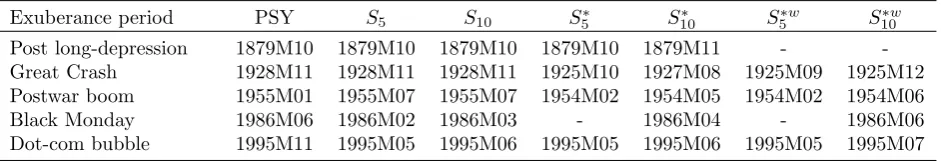
We now examine the ability of our test procedures to detect bubbles in an empirical data series.
PSY apply their real-time dating strategy (based on sequential application of a sequence of
backward recursive right-tailed DF statistics) to the S&P500 price-dividend ratio, using monthly
data over the period 1871M01-2010M12. They identify …ve primary bubble episodes: the post
long-depression period (1879M10-1880M04), the Great Crash episode (1928M11-1929M10), the
postwar boom (1955M01-1956M04), Black Monday in October 1987 (1986M06-1987M09) and
the dot-com bubble (1995M11-2001M08). Focusing on these episodes, we apply the Sm0, Sm0
and S w
m0 tests in a pseudo-real-time manner to the same dataset, beginning the testing with
the …rst 100 observations (1871M01-1879M4), to examine whether these new procedures could
have detected the onset of these bubble episodes sooner than using PSY’s approach. Table 3
reports, for each bubble episode, the …rst date for which each test rejects in favour of explosive
behaviour (the …rst of the PSY bubble regime dates is also listed for comparison in each case).
For the post long-depression, there is little to choose between theSm0 andSm0 tests, with all
of these tests …rst rejecting in either 1879M10 or 1879M11, broadly in line with the PSY date
of 1879M10. The S w
m0 tests do not detect this episode, possibly due to the reduced power of
this test when allowing for heteroskedasticity in the …nalm0 observations. For the Great Crash
episode, the Sm0 tests reject in exactly the same period identi…ed by PSY. The Sm0 and Smw0
tests reject well before this, generally in late 1925 (S10 …rst rejects in 1927M08, and S5w also rejects at this point in time as well as in 1925M10), potentially indicating an early detection
of explosive behaviour in the run-up to the Great Crash episode. In the case of the postwar
boom, the Sm0 and Smw0 tests reject several months before the initial bubble date identi…ed
by PSY. The …rst rejection is in 1954M02 for S5 and S w
5 , while rejections are …rst found in
1954M05 and 1954M06 for S10 and S10w, respectively; these are to be compared with the date of 1955M01 for PSY, demonstrating clear evidence of earlier detection of this bubble episode
(in contrast, however, the Sm0 tests only show a rejection six months after the date identi…ed
by PSY). Turning to the Black Monday period,S5 and S10 reject three to four months sooner
than PSY, S10 rejects two months earlier, and S w
10 rejects at the same time as PSY. The S5
and S5w tests fail to reject for this episode, reinforcing our overall preference for the m0 = 10
tests. Finally, for all of our proposed tests, the …rst rejections seen for the dot-com bubble are
well ahead of the date identi…ed by PSY, with S5,S5 and S5w rejecting six months before the
PSY date of 1995M11, andS10,S10andS10wrejecting four to …ve months ahead of PSY’s dates.
In addition to the exuberance periods focused on above, the Sm0, Sm0 and Smw0 tests also
reject for a number of other sequential dates across the sample period, suggesting that there
may well have been additional periods of explosive autoregressive behaviour in this series that
the newly proposed tests detect. For example, our proposed tests …nd evidence of explosive
behaviour in both the years leading up to and during the Second World War, and also …nd
the Sm0, Sm0 and Smw0 tests would in many cases have detected well-documented periods of
exuberance before the PSY approach, and also …nd evidence of some periods of explosive
be-haviour not identi…ed by PSY. This suggests a worthwhile role for the new tests, in complement
to existing procedures such as, in particular, that of PSY.
6
Conclusions
In this paper we have proposed test procedures for the detection of an end-of-sample asset
price bubble of …nite length. These involve calculating the test statistic of interest on a small
number of end-of-sample observations, with a critical value obtained by sub-sampling using the
same statistic calculated on the remaining observations. Simulation evidence highlights the size
robustness properties of our tests in …nite samples, and also their potential power advantages
when compared to existing approaches, particularly in terms of the possibility for early detection
of an ongoing end-of-sample bubble. A (pseudo) real-time monitoring exercise using the S&P500
price dividend ratio was performed, and it was found that our testing approach detected a
number of past bubble episodes a number of months in advance of the dates suggested by PSY.
As such we believe theSm0,Sm0 and Smw0 tests developed in this paper are a valuable addition
to the suite of recently developed bubble detection procedures when the focus is on early bubble
detection in a real-time setting.
References
Andrews, D.W.K. (2003). End-of-sample instability tests. Econometrica 71, 1661-1694.
Andrews, D.W.K. and Kim, J.-Y. (2006). Tests for cointegration breakdown over a short time
period. Journal of Business and Economic Statistics 24, 379-394.
Astill, S., Harvey, D.I., Leybourne, S.J. and Taylor, A.M.R. (2016). Tests for an end-of-sample
bubble in …nancial time series. Granger Centre Discussion Paper No. 16/02, School of
Economics, University of Nottingham.
Bettendorf. T. and Chen, W. (2013). Are there bubbles in the sterling-dollar exchange rate?
New evidence from sequential ADF tests. Economics Letters 120, 350-353.
Diba, B.T. and Grossman, H.I. (1988). Explosive rational bubbles in stock prices? American
Economic Review 78, 520-530.
Gilbert, C.L. (2010). Speculative in‡uence on commodity prices 2006-08. Discussion Paper
197, United Nations Conference on Trade and Development (UNCTAD), Geneva.
Harvey, D.I., Leybourne, S.J. and Sollis, R. (2016). Improving the accuracy of asset price
bubble start and end date estimators. Discussion Paper, School of Economics, University
Harvey, D.I., Leybourne, S.J., Sollis, R. and Taylor, A.M.R. (2016). Tests for explosive
…nan-cial bubbles in the presence of non-stationary volatility. Journal of Empirical Finance 38,
548-574.
Homm, U. and Breitung, J. (2012). Testing for speculative bubbles in stock markets: a
comparison of alternative methods. Journal of Financial Econometrics 10, 198-231.
Phillips, P.C.B., Wu, Y. and Yu, J. (2011). Explosive behavior in the 1990s Nasdaq: when
did exuberance escalate stock values? International Economic Review 52, 201-226.
Phillips, P.C.B., Shi, S.-P. and Yu, J. (2015). Testing for multiple bubbles: historical episodes
Table 1. Finite sample size - serial correlation
T∗= 100
θ S5 S10 R5 R10 DF5 DF10 BSADF BSADFB
−0.5 0.064 0.075 0.064 0.072 0.060 0.071 0.011 0.106
−0.3 0.067 0.081 0.066 0.076 0.060 0.070 0.040 0.127
0.0 0.069 0.086 0.067 0.081 0.061 0.068 0.073 0.148
0.3 0.071 0.088 0.069 0.083 0.061 0.067 0.066 0.193
0.5 0.072 0.088 0.069 0.083 0.060 0.067 0.055 0.208
T∗= 200
θ S5 S10 R5 R10 DF5 DF10 BSADF BSADFB
−0.5 0.057 0.062 0.056 0.061 0.057 0.059 0.007 0.055
−0.3 0.058 0.064 0.058 0.062 0.055 0.059 0.035 0.068
0.0 0.059 0.066 0.059 0.064 0.057 0.058 0.065 0.082
0.3 0.059 0.066 0.059 0.064 0.057 0.058 0.056 0.121
T a b le 2 . F in it e sa m p le si ze -v a ri a n ce sh if t T ∗ = 1 0 0 M id sa m p le L a st 5 o b se rv a tio n s σ 2 S5 S1 0 S ∗ 5 S
∗ 10
S ∗ w 5 S ∗ w 1 0 B S A D F B S A D F 1 b B S A D F 2 b S5 S1 0 S ∗ 5 S
∗ 10
S ∗ w 5 S ∗ w 1 0 B S A D F B S A D F 1 b B S A D F 2 b 1 / 1 0 0 .0 0 4 0 .0 1 3 0 .0 7 1 0 .0 8 9 0 .0 7 0 0 .0 8 6 0 .0 6 3 0 .0 6 7 0 .0 4 9 0 .0 0 0 0 .0 0 9 0 .0 6 9 0 .0 2 7 0 .0 7 0 0 .0 8 5 0 .0 2 1 0 .0 5 7 0 .0 6 2 1 / 5 0 .0 1 2 0 .0 2 4 0 .0 7 0 0 .0 8 8 0 .0 7 0 0 .0 8 6 0 .0 6 3 0 .0 6 6 0 .0 5 7 0 .0 0 2 0 .0 1 6 0 .0 6 9 0 .0 4 0 0 .0 7 0 0 .0 8 6 0 .0 2 9 0 .0 5 8 0 .0 6 2 1 0 .0 6 9 0 .0 8 6 0 .0 6 9 0 .0 8 4 0 .0 7 0 0 .0 8 5 0 .0 7 3 0 .0 6 3 0 .0 7 3 0 .0 6 9 0 .0 8 6 0 .0 6 9 0 .0 8 4 0 .0 7 0 0 .0 8 5 0 .0 7 3 0 .0 6 3 0 .0 7 3 5 0 .1 2 6 0 .1 4 7 0 .0 6 7 0 .0 8 0 0 .0 7 1 0 .0 8 5 0 .0 9 8 0 .0 6 1 0 .0 7 3 0 .2 4 7 0 .2 4 5 0 .0 6 9 0 .1 2 8 0 .0 7 0 0 .0 8 6 0 .1 6 4 0 .0 6 6 0 .1 1 1 1 0 0 .1 3 5 0 .1 5 9 0 .0 6 7 0 .0 7 9 0 .0 7 1 0 .0 8 5 0 .1 0 7 0 .0 6 0 0 .0 7 2 0 .3 1 4 0 .3 0 9 0 .0 6 9 0 .1 4 0 0 .0 7 0 0 .0 8 6 0 .2 0 8 0 .0 6 5 0 .1 2 0 T ∗ = 2 0 0 M id sa m p le L a st 5 o b se rv a tio n s σ 2 S5 S1 0 S ∗ 5 S
∗ 10
S ∗ w 5 S ∗ w 1 0 B S A D F B S A D F 1 b B S A D F 2 b S5 S1 0 S ∗ 5 S
∗ 10
[image:18.595.195.414.11.794.2]Table 3. Identified exuberance period start dates
Exuberance period PSY S5 S10 S5∗ S10∗ S∗w
5 S∗10w
Post long-depression 1879M10 1879M10 1879M10 1879M10 1879M11 -
-Great Crash 1928M11 1928M11 1928M11 1925M10 1927M08 1925M09 1925M12
Postwar boom 1955M01 1955M07 1955M07 1954M02 1954M05 1954M02 1954M06
Black Monday 1986M06 1986M02 1986M03 - 1986M04 - 1986M06
Dot-com bubble 1995M11 1995M05 1995M06 1995M05 1995M06 1995M05 1995M07
Notes: The column headed PSY records the start dates of the exuberance periods identified by Phillips, Shi and Yu (2015). The remaining columns record the first date for which a particular test rejects in favour
of a bubble. For a given window width m0 ={5,10}, Sm0 denotes our proposed Andrews-type statistic
given in equation (5),Sm∗0 denotes the studentized version given in (6) which robustifies the procedure to
volatility shifts that occur prior to the testing window, andS∗mw0 denotes the White-type corrected variant
(a)T∗= 100,m= 2 (b)T∗= 200, m= 2
(c)T∗= 100,m= 5 (d)T∗= 200, m= 5
[image:20.595.64.534.69.680.2](e)T∗= 100,m= 10 (f)T∗= 200, m= 10
Figure 1. Finite sample power of nominal 0.05-level tests: i.i.d. innovations:
(a)φ= 1.01,m0= 5 (b)φ= 1.02,m0 = 5
[image:21.595.61.536.68.467.2](c)φ= 1.01,m0= 10 (d)φ= 1.02,m0= 10
Figure 2. Rejection frequencies of nominal 0.05-level tests: single end-of-sample bubble:
Sm0: , S∗
-(a)T∗= 100,m= 2 (b)T∗= 200, m= 2
(c)T∗= 100,m= 5 (d)T∗= 200, m= 5
[image:22.595.57.535.68.682.2](e)T∗= 100,m= 10 (f)T∗= 200, m= 10
Figure 3. Finite sample power of nominal 0.05-level tests: i.i.d. innovations:
-(a) Mid sample, σ2= 1/5 (b) Mid sample,σ2= 5
[image:23.595.61.537.65.473.2](c) Last 5 observations,σ2= 1/5 (d) Last 5 observations,σ2= 5
Figure 4. Finite sample power of nominal 0.05-level tests: shift in volatility,T = 200,m= 5:
S5∗: – –,S10∗ : ,S∗w
5 : – –,S10∗w: ,BSADFb1: – –,BSADF
2