Application of machine learning for fuel consumption modelling of trucks

Application of Machine Learning for Fuel Consumption Modelling of Trucks

Federico Perrottaa_{, Tony Parry}a _{and Luis C. Neves}b

a_{University of Nottingham: Faculty of Engineering, Nottingham Transportation Engineering Centre, NTEC,}

Nottingham, United Kingdom - [email protected] - [email protected]

b_{University of Nottingham: Faculty of Engineering, Resilience Engineering Research Group, Nottingham,}

United Kingdom - [email protected]

Accepted for presentation in the 2017 IEEE International Conference on Big Data, Workshop 22 - ‘Applications of Big Data in the Transport Industry’, Dec. 11-14, 2017, Boston (MA)

Abstract - This paper presents the application of three Machine Learning techniques to fuel consumption modelling of articulated trucks for a large dataset. In particular, Support Vector Machine (SVM), Random Forest (RF), and Artificial Neural Network (ANN) models have been developed for the purpose and their performance compared. Fleet managers use telematic data to monitor the performance of their fleets and take decisions regarding maintenance of the vehicles and training of their drivers. The data, which include fuel consumption, are collected by standard sensors (SAE J1939) for modern vehicles. Data regarding the characteristics of the road come from the Highways Agency Pavement Management System (HAPMS) of Highways England, the manager of the strategic road network in the UK. Together, these data can be used to develop a new fuel consumption model, which may help fleet managers in reviewing the existing vehicle routing decisions, based on road geometry. The model would also be useful for road managers to better understand the fuel consumption of road vehicles and the influence of road geometry. Ten-fold cross-validation has been performed to train the SVM, RF, and ANN models. Results of the study shows the feasibility of using telematic data together with the information in HAPMS for the purpose of modelling fuel consumption. The study also shows that although all the three methods make it possible to develop models with good precision, the RF slightly outperforms SVM and ANN giving higher R2, and lower error.

Keywords - fuel consumption, machine learning, neural networks, random forests, support vector machine, truck fleet management

I.

INTRODUCTION

Nowadays, one of the biggest challenges to face is the reduction of greenhouse gas (GHG) emissions from the transport industry. In particular, the road transport sector accounts for about 80% of the whole energy demand required by transportation and, due to its reliance on fossil fuels, represents one of the most important sources of GHG emissions in the world [1].

Smart routing is used by fleet managers to direct their vehicles and minimise costs. Usually, the shortest path (e.g. [2]) or the least congested route (e.g. [3]) is chosen, however, some studies (e.g. [4]) showed that the road geometry and the condition of the road infrastructure can significantly affect fuel economy. A new fuel consumption model that takes into account these two factors would therefore, help fleet managers in reviewing their routing decisions. Furthermore, the model would be useful for pavement engineers and road managers to estimate the life-cycle costs of new and existing roads.

vehicles, or offer just a simplified mechanistic model. Although these capture the physical processes controlling the fuel consumption, they may be representative of only a few specific cases and may not describe what happens in reality. This is because of the assumptions made in the models. These regard the driving mode, constant speed, acceleration, weather conditions, etc. and using the same equations or methodologies in more general conditions may be computationally expensive or inaccurate due to the highly nonlinear phenomena involved.

In the era of ‘Big Data’, large quantities of data are continuously collected by companies all over the world. For example, truck fleet managers use standard sensors [8] installed on the most recent vehicles to optimize the operational costs of the fleet, for example, understanding when a vehicle needs maintenance, or a driver needs training. These are communicated using wireless telemetry and are commonly referred to as telematic data.

However, analyzing these data using traditional methods can be time consuming and computationally expensive. Moreover, when the number of data can be so large, it is difficult to select the most significant variables to include in a regression model to avoid overfitting.

Machine learning techniques are widely applied to a number of topics and represent the most advanced methods for regression problems. Among others, Support Vector Machine (SVM), Random Forests (RF), and Artificial Neural Networks (ANN) have been demonstrated to be powerful tools for regression analysis thanks to their learning ability and fault tolerance. These are applied on a daily basis to estimate, for example, the prices in the stock market (e.g. [9], [10]), hydrology (e.g. [11], [12]), and health monitoring (e.g. [13], [14]). More recently, these techniques have also been applied to estimate the fuel consumption of road vehicles (e.g. [15], [16]). However, existing studies did not use very large datasets and there is no common choice regarding the type of data to use or the variables to consider.

The aims of this paper are (1) to show an application of machine learning to Big Data for fuel consumption modelling of a large fleet of trucks, (2) to test the use of telematic and road condition data, from fleet managers and road agency databases, for fuel consumption modelling, and (3) to compare the performance of SVM, RF, and ANN in modelling the fuel consumption of large truck fleets using the available data.

II.

DATA

Truck data come from sensors installed on the most recent trucks as standard [8]. For this study, anonymized data were provided by Microlise Ltd., a company providing telematics and truck fleet management services. Only information about the performance of the trucks is available, for example the gross vehicle weight (Gross.Weight), the vehicle speed (Speed.AVG), the average acceleration (Acceleration), the geographical position (as Latitude and Longitude in WGS84), the torque percent (as Torque.Start and Torque.End), the revolutions (as Revs.Start and Revs.End in rpm) of the engine, the activation of cruise control (Cruise.Control), the use of brakes and acceleration pedal, the traveled distance (Travelled.Distance) and the fuel used (as Used.Fuel approximated to the nearest 0.001 l). Only articulated trucks are considered in this study. It is possible to identify each vehicle only by an ID number in reference to its system of sensors, the wheel configuration, and the type of engine. Date, time and an unambiguous ID number identifies each of the records. This information allows the journey of each vehicle to be retraced.

wavelengths (measured as Longitudinal Profile Variance (LPV) and named as TRACS.LPV03m, TRACS.LPV10m, and TRACS.LPV30m because measured at 3, 10, and 30 meters wavelength respectively), and the macrotexture of the road surface (measured as Sensor Measured Texture Depth (SMTD) and named as TRACS.Pav_Texture). The HAPMS is accessible online through authorization of Highways England.

This study includes records of articulated trucks travelling at a constant speed (±2.5km/h) on part of the M1 and the entire M18, two major motorways in England. The total length of the considered road segments is 300km. For the considered time window of one week, 14,281 records from 1,110 Euro 6 articulated trucks are available. Each record corresponds to a time of 60 s or a distance of 1 mile (~1609 m), whichever is shorter.

Fuel consumption (Fuel.Consumption) is calculated as the ratio between the fuel used (Used.Fuel) and the travelled distance (Travelled.Distance) transformed into l/100km.

III.

METHODOLOGY

Machine learning methods are used for regression analysis to estimate the fuel consumption of a large fleet of trucks based on telematic and HAPMS data.

The truck telematics and HAPMS were assigned to a common location reference using a GIS and an average value of each of the road characteristics was assigned to each record in the telematic database.

The dataset includes 56 variables in all. In order to avoid overfitting, among all the parameters available only the most significant have been selected and included in the regression analysis. After an initial cut-off of the variables performed by analyzing the correlation of each parameter with fuel consumption (Pearson’s correlation coefficient > 0.10) the Random Forest algorithm was used to compute variable importance [17] and among those that increase the accuracy (node purity) of the generated model, only the variables considered to have a causal effect on fuel consumption have been selected. These have been included in the regression analysis. A Support Vector Machine, a Random Forest and an Artificial Neural Network models have been developed for the estimation of fuel consumption of the considered fleet of trucks.

A. Support Vector Machine

Support Vector Machine (SVM) [18], [19] SVM is a machine learning discriminative classifier algorithm characterized by the ability to control the decision function by defining a kernel function that identifies one or multiple separating hyperplanes. Nowadays, although the mathematics behind SVM is complex [19], [20] this method is widely used in practical applications and recently, it has been used for estimating the fuel consumption of road vehicles [15].

In [15], the radial basis function (RBF) was selected as the kernel function for the SVM mode, and this has also been in this study. This is because the RBF maps samples into a higher dimensional space and can handle the case when the relation between class labels and attributes is nonlinear. The grid-search method has been used to determine the optimal parameters to use in the model. For this study, the SVM model has been developed using the e1071 R package [21]. This provides an interface to the libsvm C++ library [22] and is a powerful toolkit for SVM application.

B. Random Forest

trees in the forest. The error for the forest tends to converge as the number of trees becomes large and depends on the strength of the individual trees and the correlation between them. Because of the random processes behind it, this method is robust with respect to outliers. Furthermore, one benefit of using the RF algorithm is the possibility of using internal estimates to classify the variables due to their importance [17]. This implies the possibility of selecting the most significant variables to consider in the model, including those with nonlinear correlation, based on this algorithm.

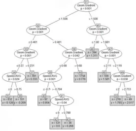
Recent studies also showed RF can be used for making predictions of the fuel consumption of road vehicles based on on-board data [16]. Today this method is widely used in various fields of science and its effectiveness has been widely proven. Many software implement the method including libraries like the randomForest R package [26], which allows the user to apply RF by defining only a few parameters such as the number of trees in the forest (ntree) and the number of features to consider and sample in each tree (mtry).

Figure 1 - Representation of part of a tree used in the developed RF model.

A higher number of trees usually implies higher precision and higher stability of the results, but also a higher computational cost. For the developed RF the number of used trees is 800 with 3 features.

C. Artificial Neural Network

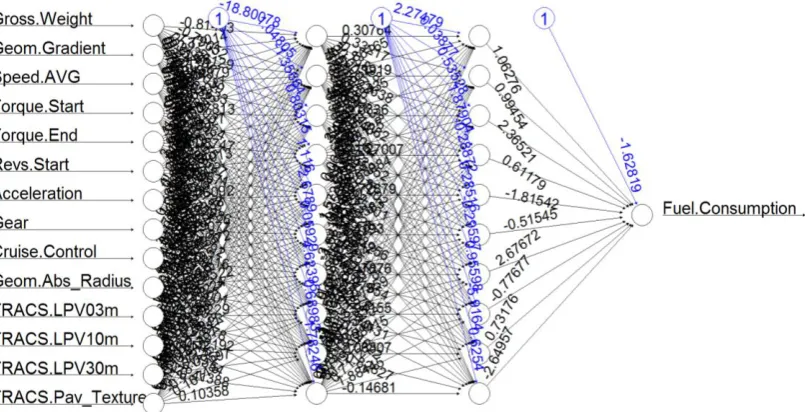
Figure 2 - Representation of the developed ANN model.

Advantages of ANN are that it requires less formal statistical training than other machine learning methods and that it is able to implicitly detect complex nonlinear relationships between explanatory variables and the response [14].

There are many different types of ANN, which use different types of neurons and activation functions. For this study, the adopted algorithm is the resilient propagation algorithm with backtracking (rprop+) [32] with logistic activation function. The developed ANN has 2 hidden layers and 10 neurons in each. This was chosen because it reduced the required calculation time and it has fewer required parameters to tune compared to others. The rprop+ neural network has been implemented by using the neuralnet R package [33].

D. Training and test

In machine learning, in order to avoid overfitting of regression models, cross-validation is usually performed. This is done by splitting the data into training and test datasets (usually 75% and 25% of data respectively) [34].

In order to define more reliable models, which make predictions independent from how the available data are subset, 10-fold cross-validation has been used in this study [34]. This means that the splitting process has been repeated randomized 10 times and 10 different models have been generated for each of the machine learning methods (SVM, RF, and ANN). The average performances, as root mean squared error (RMSE), and mean absolute error (MAE) have been used to compare the models. Obtaining similar performances of the models for each split of the data indicates that the available information is not affected by bias and that the final results are not affected by how the data are split. On the other hand, variations between data splits indicate lack of reliability of the prediction model.

IV.

RESULTS

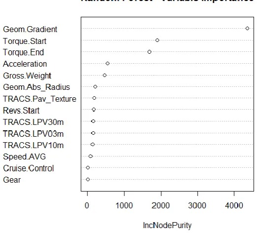
From the analysis of the Pearson’s correlation coefficients and the rank of variables made by the RF algorithm, 14 out of 56 variables initially available show significant correlation with fuel consumption (see Figure 3). These are; the gross vehicle weight (Gross.Weight); the road gradient (Geom.Gradient); the vehicle speed (Speed.AVG); the average acceleration (Acceleration); the torque % at the start of the record (Torque.Start); the torque % at the end of the record (Torque.End); the engine revs at the start of the record (Revs.Start); the used gear (Gear); the cruise control (Cruise.Control); the absolute value of the radius of curvature of the road (Geom.Abs_Radius); the road roughness as Longitudinal Profile Variance (LPV) at 3, 10, and 30 m wavelength (TRACS.LPV03m, TRACS.LPV10m, and TRACS.LPV30m respectively), and the road surface macrotexture (TRACS.Pav_Texture).

The correlation coefficient of these variables with fuel consumption is higher than 0.10 and the RF algorithm shows that including them increases the accuracy (IncNodePurity) of the resulting model. Figure 3 shows how the RF algorithm classifies the influence of the 14 selected variables on the resulting model. Because all the 14 variables increase the accuracy (and decrease the unexplained variance, IncNodePurity) of the developed models, all are included in the regression analysis to develop the SVM, RF, and ANN fuel consumption models.

From the graph representing the rank of the variables made by the RF algorithm (Figure 3), it is possible to see that the use of cruise control (Cruise.Control), the used gear (Gear), and the vehicle speed (Speed.AVG) seem to be of minor importance.

Figure 3 - Plot of variable importance for the RF algorithm.

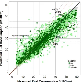
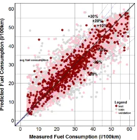
Figure 4 - Fit of the developed SVM.

Figure 6 - Fit of the developed ANN.

Figures 4, 5 and 6 show the fit of the three developed models for the training, validation and test sets for one of the 10 repetitions of the cross-validation process. In the figures the fit on the training set is represented in grey, the fit on the validation set is represented in a light color and the fit on the test set is represented in a dark color.

The following table (Table I) shows a comparison of the RMSE and MAE for the training and test sets, and the computed R2 for each of the three developed machine learning regression models.

TABLE I. Comparison of performance for the SVM, RF, and ANN models.

Model RMSE MAE R2

Support Vector Machine (SVM) 5.12 3.56 0.83

Random Forest (RF) 4.64 3.21 0.87

Artificial Neural Network (ANN) 4.88 3.46 0.85

V.

CONCLUSIONS

The study investigated the fuel consumption prediction of large fleets of trucks based on truck telematic and road geometry and condition data. Three machine learning techniques have been investigated, three models developed and their performances compared. These are a Support Vector Machine (SVM), a Random Forest (RF), and an Artificial Neural Network (ANN).

Results of the study showed that in terms of predictions, from the comparison of the RMSE, MAE, and R2, RF is the technique that gives the best performance, and this is true for both the cross-validation and testing sets. This may lead to conclusion that the RF is the best technique used to predict fuel consumption, however, the SVM and ANN demonstrated a good level of accuracy and in particular they can be considered more accurate than the RF in predicting extreme values (compare Figure 4, 5, and 6).

Although these initial results are promising, further work is required. A parametric analysis, for example, would make it possible to consider how each of the considered variables influences fuel consumption. Validation of these results for a wider range of vehicles and including more variables, such as the effect of the air temperature, wind speed, driver behavior, etc. can improve the applicability of the study. Also, it is interesting to see that the RF algorithm has included the different wavelengths of road pavement roughness and macrotexture in the variables that influence the fuel consumption of the considered fleet of trucks. This could be an important finding for the development of maintenance strategies, helping road agencies in reducing costs and greenhouse gas emissions from the road transport sector. This needs further investigation and a comparison with findings of previous studies (e.g. [4]) is recommended.

ACKNOWLEDGMENTS

This project has received funding from the European Union’s Horizon 2020 research and innovation programme under the Marie Skłodowska-Curie grant agreement No. 642453. The authors would like to thank Mohammad Mesgarpour and Ian Dickinson, from Microlise Ltd, for allowing the use of anonymized data from their databases and helping in understanding and analyzing the data, and Helen Viner, Emma Benbow, and David Peeling, from TRL Ltd, for their help in the process of extracting the data from HAPMS and interpreting part of the results of the study.

REFERENCES

[1] EPA, 2017. Inventory of U.S. Greenhouse Gas Emissionsand Sinks 1990–2015. EPA-43-P-17-001.

[2] Feillet, D., Dejax, P., Gendreau, M., and Gueguen, C., 2004. An exact algorithm for the elementary shortest path problem with resource constraints: application to some vehicle routing problems. Networks, 44 (3) (2004), pp. 216-229

[3] Fawcett J., Robinson P. Adaptive routing for road traffic. IEEE Comput. Graphics Appl. (2000) 20:46–53

[4] Chatti, K. and Zaabar, I., 2012. Estimating the Effects of Pavement Condition on Vehicle Operating Costs, National Cooperative Highway Research Program, Report no. 720. Washington, DC.

[5] Giannelli, R, Nam, E.K., Helmer, K., Younglove, T., Scora, G., Barth, M., 2005. Heavy-duty diesel vehicle fuel consumption modeling based on road load and power train parameters. SAE International, p.13. Available at: http://eprints.cert.ucr.edu/265/.

[7] Bifulco, G.N., Galante, F., Pariota, L., and Spena, M.r., 2015. A Linear Model for the Estimation of Fuel Consumption and the Impact Evaluation of Advanced Driving Assistance Systems. Sustainability, 7, 14326-14343; doi:10.3390/su71014326.

[8] SAE J1939-71, 2013. Vehicle Application Layer: Surface Vehicle Recommended Practice. SAE International. Rev. Sept. 2013.

[9] Refenes, A.N., 1993. Constructive learning and its application to currency exchange rate forecasting. In: Trippi, R.R., Turban, E. (Eds.), Neural Networks in Finance and Investing: Using Artificial Intelligence to Improve Real-World Performance. Probus Publishing Company, Chicago.

[10] Cao, L.J., and Tay, F.E.H., 2003. Support vector machine with adaptive parameters in financial time series forecasting, IEEE Transactions on Neural Network, vol. 14, no. 6, pp. 1506-1518.

[11] Khan and Coulibaly, 2006. Application of support vector machine in lake water level prediction. Journal of Hydrologic Engineering, 11 (3), pp. 199-205.

[12] Herrera, M., Torgo, L., Izquierdo, J., and Pérez-García, R., 2010. Predictive models for forecasting hourly urban water demand, J. Hydrol., 387, 141–150.

[13] Burke, H.B., 1994. Artificial neural networks for cancer research: Outcome prediction, Sem. Surg. Oncol., vol. 10, pp. 73-79.

[14] Tu, J.V., 1996. Advantages and disadvantages of using artificial neural networks versus logistic regression for predicting medical outcomes. Journal of Clinical Epidemiology, 49 (11), pp. 1225-1231.

[15] Zeng, W., Miwa, T. & Morikawa, T., 2015. Exploring trip fuel consumption by machine learning from GPS and CAN bus data. Journal of the Eastern Asia Society for Transportation Studies, 11(June 2016), pp.906–921.

[16] Almér, H., 2015. Machine learning and statistical analysis in fuel consumption prediction for heavy vehicles. KTH, Sweden.

[17] Breiman, L., 2001. Random forests. Machine Learning, 45(1), pp.5–32.

[18] Cortes, C. and Vapnik, V., 1995. Support-vector network. Machine Learning, 20, 1–25.

[19] Vapnik, V., 1998. Statistical learning theory. New York: Wiley.

[20] Gunn, S.R., 1998. Support Vector Machines for Classification and Regression. Technical Report. Faculty of Engineering, Science and Mathematics, School of Electronics and Computer Science. University of Southampton. Southampton, UK.

[21] Meyer, D., Dimitriadou, E., Hornik, K., Weingessel, A., & Leisch, F. et al. 2017, e1071: Misc Functions of the Department of Statistics, Probability Theory Group 13 (Formerly: E1071), TU Wien, R package version 1.6-8.

[22] Chang, C.C. and Lin, C.J., 2001. LIBSVM: a library for support vector machines. Software available at http://www.csie.ntu.edu.tw/-~cjlin/libsvm, detailed documentation (algori-thms, formulae) can be found at: http: //www.csie.ntu.edu.tw/~cjlin/papers/libsvm.ps.gz.

[23] Breiman, L., Friedman, J.H., Olshen, R.A., Stone, C.J., 1984. Classification and Regression Trees. Wadsworth; Belmont, California.

[25] Khaidem, L., Saha, S., Dey, S.R., 2016. Predicting the direction of stock market prices using random forest, CoRR. Available at: http://arxiv.org/abs/1605.00003.

[26] Liaw, A., Wiener, M., Breiman, L., and Cutler, A., 2015. Breiman and Cutler's Random Forests for Classification and Regression. (Formerly: ‘randomForest’). R package ver. 4.6-12.

[27] McCulloch, W., Pitts, W., 1943. A Logical Calculus of Ideas Immanent in Nervous Activity. Bulletin of Mathematical Biophysics. 5 (4): 115–133. doi:10.1007/BF02478259.

[28] Werbos, P.J., 1975. Beyond Regression: New Tools for Prediction and Analysis in the Behavioral Sciences.

[29] Stergiou, C. and Siganos, D., 1995. Neural Networks. Available at: https://www.doc.ic.ac.uk/-~nd/surprise_96/journal/vol4/cs11/report.html#What is a Neural Network [Accessed October 4, 2016].

[30] Schilling, G.D., 1997. Modeling Aircraft Fuel Consumption with a Neural Network. Computer Science.

[31] Trani, A.A. et al., 2004. A Neural Network Model to Estimate Aircraft Fuel Consumption. In AIAA 4th Aviation Technology, Integration and Operations (ATIO) Forum. Chicago, Illinois: American Institute of Aeronautics and Astronautics, p. 24.

[32] Riedmiller, M., 1994. Rprop – Description and Implementation Details. Technical report.

[33] Fritsch, S., Guenther F., Suling, M. and Mueller, S.M., 2016. Training of Neural Network. (Formerly: neuralnet). R package ver. 1.33.