Noise Parameter Estimation
for Non-Singleton Fuzzy Logic Systems
Direnc Pekaslan, Jonathan M. Garibaldi and Christian Wagner
Intelligent Modelling and Analysis Group (IMA),Lab for Uncertainty in Data and Decision Making (LUCID), School of Computer Science,University of Nottingham,
Nottingham, NG8 1BB, UK
{direnc.pekaslan, jon.garibaldi, christian.wagner}@nottingham.ac.uk
Abstract—Real-world environments face a wide range of noise (uncertainty) sources and gaining insight into the level of noise is a critical part of many applications. While Non-Singleton Fuzzy Logic Systems (NSFLSs), in particular recently introduced advanced variants such as centroid-based NSFLSs have the capacity to handle known quantities of uncertainty, thus far, the actual level of uncertainty has had to be defined a priori - i.e. prior to run time of a system or controller. This paper does not focus on such advances within the architecture of NSFLSs, but focuses on a novel two-stage approach for uncertainty handling in fuzzy logic systems which integrates: (i) estimation of noise levels and (ii) the appropriate handling of the noise based on this estimate, by means of a dynamically configured NSFLS. As initial evaluation of the approach, two chaotic nonlinear time series (Mackey-Glass and Lorenz), as well as a real-world Darwin sea level pressure series prediction fuzzy logic systems are implemented and compared to commonly used procedures. The results indicate that the proposed strategy of integrating uncer-tainty/noise estimation with the capacity of non-singleton fuzzy logic systems has the potential to deliver performance benefits in real-world applications without requiring a priori information on noise levels and thus delivers a first step towards smart, noise-adaptive non-singleton fuzzy logic systems and controllers.
I. INTRODUCTION
Noise (uncertainty) can be defined as an undesirable random distortion in data and it is present in most real-world circum-stances including (but not limited to) sensors, images, speech or time series etc. As real-world environments, such as in control, face a wide range of noise sources, gaining insight into the level of noise becomes a critical part of many applications. Therefore, noise studies are attracting considerable interest in terms of the accurate estimation and/or removal of noise from data. Due to the broad variance in noise levels in different real-world circumstances, an accurate noise estimation can be a challenging task. As a result, the removal of estimated noise from a dataset can risk being either an ineffective, or in some cases even detrimental, approach. In light of this, while the es-timation of noise is a crucial initial step for many applications, it may be beneficial to consider an alternative approach which avoids noise removal in favour of robustly handling uncertainty and noise as part of the control of decision making algorithms. Fuzzy set (FS) theory was first introduced by Zadeh [1] and provided the basis for Fuzzy Logical Systems (FLSs) which are considered as robust systems to capture noise in decision making. FLSs processes are completed in three
essential steps; fuzzification, inferencing and defuzzification. In fuzzification, crisp input values are transformed into FSs and this transformation can be implemented as a singleton (SFLSs) or non-singleton (NSFLSs). Due to the fact that inputs are commonly corrupted by noise, non-singleton fuzzy sets have potentially designed to capture the existed noise in input data, and so may provide better results than SFLSs for the same number of rules [2]–[7]. To illustrate uncertainty handling with the non-singleton designs, the extensive studies in time series prediction are carried out [6], [8]–[16]. In these studies, it is assumed that the additive noise level (σnoise) is
already either a priori known or can be calculated by using the known values of the signal to noise ratio (SNR) and standard deviations of a noise free set (σnf). After ascertaining
the σnoise value, this is utilised as the parameters for
non-singleton input MFs in NSFLSs. Then the various further adjustments (such as optimisation) are/are not implemented and the remaining fuzzy procedures are performed. However, the prior knowledge of additive noise level (σnoise) may
not reflect real-world situations, in which the level of noise information cannot be obtained in advance.
focus on such advances within the architecture of NSFLSs, but focuses on specifically one key problem detecting noise levels to define NSFLSs parameters at run time.
Since the generation of nonlinear time series samples is an easily manageable procedure and different noise levels can be injected in a controlled manner, this paper focuses on time series prediction rather than for example real world control. As the proposed strategy of integrating uncertainty/noise estimation with the capacity of NSFLSs has the potential to deliver performance benefits without requiring a priori information on noise levels, it can be applied to a wide range of real-world control applications which contains uncertainty from robotics to unmanned aerial vehicle (UAV) control.
The structure of this paper is as follows. Section II gives a brief overview of singleton, non-singleton FSs and time series datasets along with noise adding procedures. Section III introduces each step of the experiment including the noise estimation technique. The next Section IV gives detail of the experimental environment, the results and discussion. In Section V, the conclusions of experiments with possible future work directions are given.
II. BACKGROUND
In this section, a brief explanation of singleton, non-singleton fuzzy sets will be introduced and an overview of time series datasets with noise adding procedures will be given.
A. Singleton and Non-singleton Fuzzy Logic Systems
In standard singleton fuzzification, a given crisp inputxis transformed into an input fuzzy set Iwhich is represented by a membership function µI(x)that takes values in the interval
[0,1], formulated as:
I={x,(µI(x))| ∀x∈X} (1)
Singleton sets are characterised by a single point inIhaving the value of 1:
µI(xi) =
(
1 xi=x0i,
0 xi6=x0i,
(2)
In non-singleton fuzzification step, after identifying noise level, it is processed on input data (x) by transforming it to an MF. Normally it is assumed that the incoming input xis the value which is possibly to be real and because of existing noise, it is assumed that neighbour values of the xhave also potential to be real values. However, as we go further from the input xvalue, the possibility of being real value getting less and less in which expressed non-singleton MFs. Hence it can be said that non-singleton MFs have a potential to capture sys-tem uncertainty in an efficient manner. When the non-singleton fuzzifier is considered, the crisp input transformation to fuzzy sets can be formed in numerous shapes and as a sample, non-singleton Gaussian input MF is formulated as follows:
µI(xi) = exp
"
−1
2
x −xi
σnoise
2#
(3)
wherex0i is the crisp value of the input andσnoiseis the noise
level of system.
B. Time Series
In our experiment artificially generated Mackey-Glass [17], Lorenz [18] time series, which exhibits chaotic behaviour, have been chosen to be tested. In addition that, the real-world Darwin sea level pressure series is also been used to test noise estimation and capturing capability of our system.
1) Mackey-Glass Time series: The Mackey-Glass equation is the nonlinear time delay differential equation which is formulated as:
dx(t) dx =
ax(t−τ)
1 +x10(t−τ)−bx(t) (4)
where a, b and n are constant real numbers, t is the current time and τ is the delay time.
2) Lorenz Time series: The Lorenz Time series was derived from a model of the earth’s atmospheric convection flow heated from below and cooled from above and it is described using nonlinear differential equations as follows [18]:
˙
x=σ(y−x) y˙ =x(p−z)−y z˙=xy−bz (5)
where the dots denote the next values to the three variables x, y, zin the time series.
3) Darwin sea level pressures: Monthly values of the Darwin Sea Level Pressure series are gathered between 1882-1998. The dataset consists of 1300 samples and it can be obtained from (http://research.cs.aalto.fi).
C. Noise Adding to Time Series
The noise is measured by signal-to-noise ratio (SNR) and while high SNR values refer to less noise, low SNR values refer to a high level of noise in a dataset. SNR calculation is done as follows:
SN R= 10∗log( σ
2
nf
σ2
noise
) (6)
whereσnf is the standard deviation of noise free dataset.
The Gaussian noise adding procedure is implemented based on the SNR values below:
By deriving the formula above, σnoise value can be
gathered:
σnoise=
σnf
10(SN R
20 )
(7)
Then random noise values, with 0 mean, are added to the noise free values as follows:
xt→xt+N(0, σ2noise) (8)
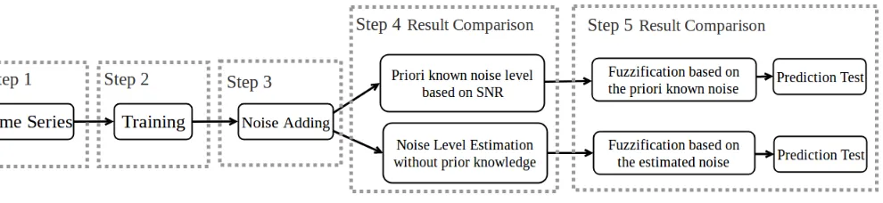
Fig. 1: A Flow chart of the experiment procedures
III. METHODOLOGY
In the literature, there are a number of studies which deal with uncertainty in time series data by means of NSFLSs [6], [8]–[16]. Generally, it is assumed that noise levels (σnoise) are
known in advance or it is calculated by using the known SNR andσnf values (7). Thereafter, non-singleton input parameters
in the NSFLSs are defined based on theσnoiseand further
pro-cedures such as optimisation etc. may/may not be carried out. In this paper, firstly, a noise estimation technique is applied to the noisy time series and it is compared to the priori known noise levels. Moreover, the estimated noise levels are captured in NSFLSs and prediction results are provided. Due to the fact that real-world environments face a wide range of non-stationary noise sources, the dynamic estimation of noise levels and capturing it in a fuzzy system potentially has features to a different variety of applications, which possibly contain noise, such as sensor studies, stock market forecasting or signal processing and etc.
The methodology of the current work can be divided into five main steps and it is illustrated in the flow chart (Fig. 1); Step 1 Time Series: The procedures in Section II-B are followed to generate chaotic time series datasets. In addition to the artificially generated time series, a real-world Darwin sea level pressure dataset is tested in the experiment.
Step 2 Training: As the training phase of FLSs, the rule generation is completed by utilising Wang-Mendel method [19] over the first 70% of the data points (noise free training set) in the total time series for MG, Lorenz and sea level pressure series.
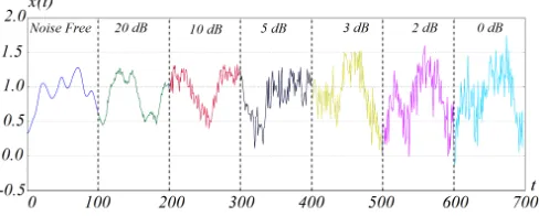
Step 3 Noise Injection: The procedures of Section II-C are followed to add Gaussian noise to the time series datasets. Since the real-world may contain different levels of noise, in order to imitate real-world circumstances and analyse our proposed method, six different noise levels (from low to high) are employed per experiment.
Step 4 Noise Identification:At this step of the experiment, two different procedures are performed. Firstly, an estimation technique is performed to identify noise level and secondly, the traditional procedures (the priori known parameters) are used to calculate noise levels:
1) Noise Level Estimation without prior knowledge: In literature, there are the numerous number of noise estimation techniques which could be used in this study [20]–[24]. However, as an initial step of this work, one of the initial noise estimation study for images [25] is performed to estimate
noise of time series dataset. In the study [25], firstly, difference operator is implemented over image patches and standard deviation of differenced patches is calculated. Thereafter, a histogram is evaluated in order to receive desired noise level estimationσnoise.
In this work, for the sake of simplicity and unconcerned of patch parameters, the whole time series is considered as one patch and difference operator is conducted as follows:
y(t)=
1
√
2(x(t+1)−x(t)) t= 1,2,3....N (9)
Then, the variance of the differenced setyis calculated and theσnoise is gathered:
σnoise=
v u u t
1 N
N
X
t
yt (10)
By following 9 and 10, noise estimation is completed without any prior knowledge and the estimated noise levels can be used to dynamically define parameters for non-singleton input MFs in the fuzzification part of NSFLSs.
2) A Priori Known Noise Level Identification: The additive noise to the noise free time series set is represented asσnoise
and in the literature, generally, it is assumed that the σnoise
is already known or we have the information aboutSN Rand variance of noise free set(σnf). So that the noise levelσnoise
can be calculated as it is shown in (7).
The first result comparison between the estimated and the priori known noise levels is done as it is pointed out in Step 4 of the Fig. 1.
Step 5 Prediction Test:The remained 30% of the time series are used to test NSFLSs. In the fuzzification of NSFLSs testing process, firstly, the estimated noise levels are used as the (adaptive) standard deviation of Gaussian input MFs and the NSFLS prediction test is performed. Then the same experiment is repeated; however this time priori known noise level is used in the fuzzification step to define input MFs.
Fig. 2: An illustration of the used antecedents MFs in training.
As mentioned earlier, rather using advanced architecture NSFLSs, such as centroid or similarity based systems [6], [15], [16], in the inference step of FLSs, the standard minimum t-norm and max t-conorm operators are used and centroid defuzzification is utilised in the last step of FLSs. The same number of discretisation level (500) is used for all FLSs. In order to mitigate the effect of randomness in the noise addition process, each experiment is repeated 30 times for all case scenarios and the average of generated Mean Square Errors (MSEs) were calculated.
IV. EXPERIMENT ANDRESULT
A. Time Series Datasets and Training
The experiment is performed on three different time series data. As the Step 1 of the experiment, first, Mackey Glass (MG) and Lorenz time series datasets are generated and in order to provide a chaotic behaviour, τ is set to 30, while a= 0.2 andb = 0.1 for MG (4) and the Lorenz time series parameters are set as σ=10, b=8/3 and p=28 (5). x(t) are generated for 2000 time points (from t=-999 to t=1000) and due to the fluctuation tendency in the initial part of the time series, the last1000(fromt=1 tot=1000) points are taken to be used in the experiment. Second, monthly data of sea level pressure in Darwin, which consist 1300 samples, is obtained from (http://research.cs.aalto.fi/) and used in the experiment.
As the Step 2 of the experiments, training is implemented by using Wang-Mendel technique [19] and during rule creation, seven antecedents MFs (See Fig. 2) are created as left shoulder, 5 equally distributed triangular and right shoulder antecedents. Nine past points were projected to the corresponding an-tecedents and the following (10th) point was designated as the output. The window sliding procedure is applied until reaching the end of the training set.
B. Noise Adding
After the FLS rule generation is completed by using noise free set, the datasets are distorted by noise (as in Step 3) to test our approach under different circumstances. Six different Gaussian noise SNR levels (0,2,3,5,10 and 20 dB) were injected to MG, Lorenz and sea level pressure data to be used in different variations of the experiment (a sample of noise differences can be seen in Fig. 3).
C. Noise Level Identification
As can be seen in Step 4 of the Fig. 1, two different noise level determination strategies are implemented:
Fig. 3: The sample of different noise levels on Mackey-Glass Time series dataset
1) Noise estimation without prior knowledge: In this esti-mation, it is assumed that there is no any prior information (neither SNR norσnf) and the noise level estimation is carried
out on the testing set. For each set (with different noise levels), the procedures in the Section III-1 are followed to estimate noise levels. First, the difference operator for the test set is performed and second, the standard deviation (σnoise) of the
differenced vector is defined as the noise level in the set. 2) Noise Level calculation with prior knowledge: In this technique, as it is carried out in the literature [6], [8]–[16], it is presumed that the standard deviation (σnf) of noise free
set (first 70% of the data) and SNR values for each variation of experiment is already known in advance. By following the (7), the standard deviation (σnoise) is calculated to define noise
level of the set and it is used to define input MF parameter in the fuzzification of non-singleton input MFs.
D. Result Comparison for Noise Level Identification
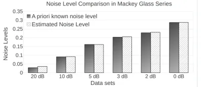
In this section, noise estimation (see section IV-C1) and the priori known noise level (see section IV-C2) comparison result is given under six different noisy dataset. As the noise adding procedures is practised 30 times for each noise level, the average of estimation are given. The xaxes of the Figs. 4, 5 and 6 below represent noise levels in dBs and the y axes represent the calculated variance (σnoise). The figures
compares result for the noise calculations and the estimation under six different SNR values for MG, Lorenz and sea level pressure respectively.
E. Result Comparison for Time Series Prediction
In this section, the previously estimated and priori known noise levels are adopted in the input MFs of the NSFLSs and the average MSE prediction results are compared in regards to both noise estimation and the known noise level calculation (as inStep5). Figs. 7, 8 and 9 shows the prediction MSE result for Mackey Glass, Lorenz time series and sea level pressure data respectively. Note that as each variation of the experiment is repeated 30 times, the average MSE results are provided in these figures.
F. Discussion
[image:4.612.316.560.56.154.2]Fig. 4: Mackey Glass noise levels comparison between the priori known and estimated (without prior knowledge)
[image:5.612.79.275.172.255.2]Fig. 5: Lorenz series noise levels comparison between the priori known and estimated (without any prior knowledge)
Fig. 6: Darwin sea level pressure time series noise levels comparison between the priori known and estimated (without any prior knowledge)
different noise levels. The performance of each noise level identification is provided in Figs. 4, 5 and 6 for MG, Lorenz and sea level pressure data respectively. Thereafter, both the priori known and estimated noise levels are used to define input MFs of the fuzzy system and corresponding MSEs results are provided in Figs. 7, 8 and 9. Note that noise in the data are able to be handled by tuning the parameters of the input MFs of NSFLSs based on the noise estimation.
Figures 4 and 5 show that the noise levels in the time series can be estimated without prior knowledge and it can be said that the estimation levels are consistent with priori known noise levels. Further, when the estimated levels are proceeded to NSFLSs, as it is expected, the MSEs results of prediction is in a complete agreement with the priori known noise level predictions (Figs. 7 and 8).
Further analysis in noise estimation is implemented in the real-world seal level pressure data. It should be noted that due to the fact that there are a tremendous number of uncertainty source in the real-world application, finding a generally applicable and accurate noise level estimation technique may not be realistic. To that end, when the noise estimation technique is performed without prior knowledge of dataset, it can be clearly seen in Fig. 6 that there is a strong discrepancy between priori known and estimated noise levels as it may be expected. As the further step of the experiment,
[image:5.612.339.542.187.272.2]Fig. 7: Mackey Glass time series average MSE for prediction comparison between the priori known and estimated noise levels in input MFs
Fig. 8: Lorenz time series average MSE for prediction com-parison between the priori known and estimated noise levels in input MFs
Fig. 9: Darwin Sea Level Pressure time series average MSE for prediction comparison between the priori known and estimated noise levels in input MFs
priori known and estimated noise levels are proceeded to NSFLS, regardless of the inaccuracy in the noise estimation. Despite the fact that, noise estimation could not be performed accurately, surprisingly the MSEs result comparison in Fig. 9 shows that the strong discrepancy is relatively disappeared when the noise levels are proceed to NSFLSs.
[image:5.612.78.275.293.371.2] [image:5.612.336.543.322.405.2]the NSFLSs is utilised for the priori known and estimated noise levels, it is observed that under low level of noises (20 and 10 dB), the inaccuracy of the estimation is reduced significantly based on the paired two sample t-test. Moreover, as can be clearly seen in the Fig. 6, the noise estimation is not made to be close to priori known noise levels. However when the traditional and estimated noises are used as parameters in NSFLSs, based on paired two sample t-test, it is observed that the impact of error in noise estimation is reduced significantly under each level (20, 10, 5, 3, 2 and 0 dBs) of noise.
Based on above, it can be said that the strategy of focus-ing on detectfocus-ing noise levels -without prior knowledge- and using the estimation to define the non-singleton parameters dynamically has strong potential to mitigate the impact of noise/uncertainty in real world systems.
V. CONCLUSION
In this paper, two different aspects are investigated; (i) first, a method of noise level estimation that can be implemented without any prior knowledge about the dataset (ii) second, the effects of preserving estimated noise levels and using these to define NSFLSs parameters. This technique allows for the construction of dynamically parametrised NSFLSs, which can handle the noise in the system without requiring any information regarding the prior stage of dataset. The experiment is implemented on two commonly used chaotic time series (Mackey-Glass and Lorenz Time series) and on a real-world sea level pressure dataset. The evidence from this study suggests that noise level estimation can be implemented without any prior information about the dataset, and a possible impact of the erroneous risk in the estimation can be alleviated by capturing and handling noise in NSFLSs. In the light of this, the NSFLS based proposed strategy could indeed be a suitable approach to be used in a wide range of real-world control applications with different levels of non-stationary noise.
Future work will concentrate on different noise estimation techniques and their impact in respect to the different advanced NSFLS architectures such as centroid or similarity based NSFLSs. Further, we will explore the real-world utility of the proposed approach in both simulated and real-world control experiments, for using on robotic case studies. Lastly, due to the increased modelling capabilities of type-2 fuzzy logic in handling uncertainty, different type-2 designs will be explored.
ACKNOWLEDGMENT
This paper was partially supported by the UK EPSRC grant EP/P011918/1.
REFERENCES
[1] L. A. Zadeh, “Fuzzy sets,”Information and control, vol. 8, no. 3, pp. 338–353, 1965.
[2] M. Balazinski, E. Czogala, and T. Sadowski, “Control of metal-cutting process using neural fuzzy controller,” inFuzzy Systems, 1993., Second IEEE International Conference on. IEEE, 1993, pp. 161–166. [3] Y. Hayashi, J. J. Buckley, and E. Czogala, “Fuzzy neural network with
fuzzy signals and weights,”International Journal of Intelligent Systems, vol. 8, no. 4, pp. 527–537, 1993.
[4] P. M. Larsen, “Industrial applications of fuzzy logic control,” Interna-tional Journal of Man-Machine Studies, vol. 12, no. 1, pp. 3–10, 1980.
[5] N. Sahab and H. Hagras, “A hybrid approach to modeling input variables in non-singleton type-2 fuzzy logic systems,” in2010 UK Workshop on Computational Intelligence (UKCI), Sept 2010, pp. 1–6.
[6] C. Wagner, A. Pourabdollah, J. McCulloch, R. John, and J. M. Garibaldi, “A similarity-based inference engine for non-singleton fuzzy logic systems,” in Fuzzy Systems (FUZZ-IEEE), 2016 IEEE International Conference on. IEEE, 2016, pp. 316–323.
[7] A. B. Cara, C. Wagner, H. Hagras, H. Pomares, and I. Rojas, “Mul-tiobjective optimization and comparison of nonsingleton type-1 and singleton interval type-2 fuzzy logic systems,” IEEE Transactions on Fuzzy Systems, vol. 21, no. 3, pp. 459–476, 2013.
[8] G. C. Mouzouris and J. M. Mendel, “Dynamic non-singleton fuzzy logic systems for nonlinear modeling,”IEEE Transactions on Fuzzy Systems, vol. 5, no. 2, pp. 199–208, May 1997.
[9] J. M. Mendel, “Uncertainty, fuzzy logic, and signal processing,”Signal Processing, vol. 80, no. 6, pp. 913 – 933, 2000. [Online]. Available: http://www.sciencedirect.com/science/article/pii/S0165168400000116 [10] Q. Liang and J. M. Mendel, “Equalization of nonlinear time-varying
channels using type-2 fuzzy adaptive filters,” IEEE Transactions on Fuzzy Systems, vol. 8, no. 5, pp. 551–563, Oct 2000.
[11] S. Jafarinezhad and M. Shahbazian, “System identification of a non-linear continuous stirred tank heater based on type-2 fuzzy system,” in
2011 Chinese Control and Decision Conference (CCDC), May 2011, pp. 1869–1874.
[12] Y. Chen, D. Wang, and S. Tong, “Forecasting studies by designing mamdani interval type-2 fuzzy logic systems: With the combination of bp algorithms and km algorithms,”
Neurocomputing, vol. 174, pp. 1133 – 1146, 2016. [Online]. Available: http://www.sciencedirect.com/science/article/pii/S0925231215014915 [13] G. C. Mouzouris and J. M. Mendel, “Nonsingleton fuzzy logic systems:
theory and application,”IEEE Transactions on Fuzzy Systems, vol. 5, no. 1, pp. 56–71, Feb 1997.
[14] J. M. Mendel,Uncertain rule-based fuzzy logic systems: introduction and new directions. Prentice Hall PTR Upper Saddle River, 2001. [15] A. Pourabdollah, C. Wagner, J. H. Aladi, and J. M. Garibaldi, “Improved
uncertainty capture for nonsingleton fuzzy systems,”IEEE Transactions on Fuzzy Systems, vol. 24, no. 6, pp. 1513–1524, Dec 2016.
[16] D. Pekaslan, S. Kabir, J. M. Garibaldi, and C. Wagner, “Determining firing strengths through a novel similarity measure to enhance uncer-tainty handling in non-singleton fuzzy logic systems,” inInternational Joint conference on computational Intelligence (IJCCI), 2017. [17] M. C. Mackey, L. Glasset al., “Oscillation and chaos in physiological
control systems,”Science, vol. 197, no. 4300, pp. 287–289, 1977. [18] E. N. Lorenz, “Deterministic nonperiodic flow,”Journal of the
atmo-spheric sciences, vol. 20, no. 2, pp. 130–141, 1963.
[19] L.-X. Wang and J. M. Mendel, “Generating fuzzy rules by learning from examples,”IEEE Transactions on systems, man, and cybernetics, vol. 22, no. 6, pp. 1414–1427, 1992.
[20] C.-T. Lin, “Single-channel speech enhancement in variable noise-level environment,” IEEE Transactions on Systems, Man, and Cybernetics-Part A: Systems and Humans, vol. 33, no. 1, pp. 137–143, 2003. [21] G. D. Wu and C. T. Lin, “A recurrent neural fuzzy network for
word boundary detection in variable noise-level environments,” IEEE Transactions on Systems, Man, and Cybernetics, Part B: Cybernetics, vol. 31, no. 1, p. 8497, 2001.
[22] J. Biemond and J. J. Gerbrands, “An edge-preserving recursive noise-smoothing algorithm for image data,” IEEE Transactions on Systems, Man, and Cybernetics, vol. 9, no. 10, pp. 622–627, Oct 1979. [23] O. Renaud, J. L. Starck, and F. Murtagh, “Wavelet-based combined
signal filtering and prediction,” IEEE Transactions on Systems, Man, and Cybernetics, Part B (Cybernetics), vol. 35, no. 6, pp. 1241–1251, Dec 2005.
[24] M. A. Khanesar, E. Kayacan, M. Teshnehlab, and O. Kaynak, “Analysis of the noise reduction property of type-2 fuzzy logic systems using a novel type-2 membership function,”IEEE Transactions on Systems, Man, and Cybernetics, Part B (Cybernetics), vol. 41, no. 5, pp. 1395– 1406, Oct 2011.