Murray polygons as a tool in image processing

MURRAY POLYGONS AS A TOOL IN IMAGE PROCESSING

Bhuwan Pharasi

A Thesis Submitted for the Degree of PhD

at the

University of St Andrews

1990

Full metadata for this item is available in

St Andrews Research Repository

at:

http://research-repository.st-andrews.ac.uk/

Please use this identifier to cite or link to this item:

http://hdl.handle.net/10023/13580

Murray Polygons as a Tool in

Image Processing

thesis submitted

in fulfilment for the requirement of

the degree of

DOCTOR OF PHILOSOPHY

by

Bhuwan Pharasi.

Department of Computational Sciences,

University of St. Andrews

St. Andrews

ProQuest Num ber: 10166334

All rights reserved

INFORMATION TO ALL USERS

The quality of this reproduction is dependent upon the quality of the copy submitted.

In the unlikely event that the author did not send a com plete manuscript

and there are missing pages, these will be noted. Also, if material had to be removed, a note will indicate the deletion.

uest

ProQuest 10166334

Published by ProQuest LLO (2017). Copyright of the Dissertation is held by the Author.

All rights reserved.

This work is protected against unauthorized copying under Title 17, United States C ode Microform Edition © ProQuest LLC.

ProQuest LLC.

789 East Eisenhower Parkway P.Q. Box 1346

I:

To my mother Smt Sumitra Devi Pharasi and my father Sh. Mangla Nand Pharasi

I Bhuwan Pharasi hereby certify that this thesis has been composed by

myself, that it is a record of my own work, and that it has not been accepted in partial or complete fulfilment of any other degree or professional

qualification.

Signed... D a te .1

I was admitted to the Faculty of Science of the University of St.Andrews under Ordinance General No 12 on October 10.1986 and as a candidate for the degree of Ph.D on October 10. 1987.

Signed... Date...

I hereby certify that the candidate has fulfilled the conditions of the Resolutions and Regulations appropriate to the degree of Ph.D.

Signature of Supervisor ... Date ...

QsmmM

In submitting this thesis to the University of St. Andrews I understand that I am giving permission for it to be made available for use in accordance with the regulations of the University Library for the time being in force, subject

to any copyright vested in the work not being affected thereby. I also

Acknowledgements

It gives me an immence pleasure and great opportunity to express my profound sense of gratitude and indebtedness to Professor A. J. Cole, for his painstaking guidance, invaluable suggestions and constant

encouragement throughout the research work.

I wish to express my thanks to Professor R. Morrison; Chairman, for providing all necessary facilities and also to Dr. J. Owczarczyk for proof­ read and helping me during this project.

I also wish to record my appreciation and feeling of gratitude to Mr.

A. J. T. Davie, Dr. A. Brown, Dr. R. Dyckhoff, Mrs. H. Bremner, Mrs. E. Nicoll and Mr. B. McAndie who helped me in every possible way.

My humble regards are also due to my others family members who have always encouraged and assisted me to pursue higher studies.

I am also thankful to: the Committee of Vice-Chancellors and Principals, and St. Andrews University, for providing me the financial

support.

Abstract

This thesis reports on some applications of murray polygons, which are a generalization of space filling curves and of Peano polygons in

particular, to process digital image data. Murray techniques have been used on

2-dimensional and 3-dimensional images, which are in cartesian/polar

co-ordinates. Attempts have been made to resolve many associated aspects of

image processing, such as connected components labelling, hidden surface removal, scaling, shading, set operations, smoothing, superimposition of images, and scan conversion.

Initially different techniques which involve quadtree, octree, and linear run length encoding, for processing images are reviewed. Several image

processing problems which are solved using different techniques are described In detail. The steps of the development from Peano polygons via multiple radix

arithmetic to murray polygons is described. The outline of a software

implementation of the basic and fast algorithms are given and some hints for a hardware implementation are described

The application of murray polygons to scan arbitrary images is explained. The use of murray run length encodings to resolve some image

processing problems is described. The problem of finding connected components, scaling an image, hidden surface removal, shading, set

operations, superimposition of images, and scan conversion are discussed.

Most of the operations described in this work are on murray run lengths. Some operations on the images themselves are explained.

quadtrees, and octrees. All the algorithms obtained using murray scan

CONTENTS

INTR O D UCTIO N X

A

1 -1 Introduction 1

1 - 2 Run-Length Encoding 3 !

Linear Scan 5

Space Filling Curves 6

1 - 3 Quadtree Encoding 9

Leaf Node 1 2

Traversal Of The Node Of Its Quadtree 1 5

1 - 4 Volume Data 16

2 . M URRAY POLYGONS 2 0

2 - 1 Introdution 20

2 - 2 Murray Polygons 2 0

. Gray Codes or Cyclic Progressive Numbers 2 3

Direct Peano Transformations 2 5

Murray Arithmetic 2 6

Murray Transformation 2 8

Mixed Scan 3 1

Some Lemmas 32

Implementation Of Murray Scan 3 9

Original Implementation 3 9

A Faster Murray Scan Algorithm 4 2

Hardware Implementation 4 6

Three-Dimensional Cartesian Coordinates 4 6

Extension To 3-D And n-D Murray Polygons 4 7

Method One 4 7

Some Lemmas 5 0

Second Method 5 2 ■

Polar Murray Scan 54 }

Polar Coordinates 5 4

I

Changing Coordinates Systems 5 5

Graphs In Polar Coordinates 5 6 |

Cylindrical And Spherical Coordinates 5 6

Implementation Of Planar Polar Murray Scan 5 9

Cylindrical Polar Murray Scan 6 1

Spherical Polar Murray Scan 6 1

2-2.11 Application Areas 62

Scanning 6 2

2-2 .1 2 Remarks 63

3 . SCANMNG AND DRAW ING OF TH E IM AGES 6 4

3 -1 Introduction 6 4

3 - 2 Structure And List Processing 6 5

3 - 3 Linked List 68

3-4 Image Construction 69

3-5 Storing an Image in a Database 7 2

Retrieving an Image From a Database 7 4

3 - 6 Scanning And Drawing Of An Image 74

3 - 7 Remarks 8 o

4 . SCAN CONVERSION AND SCALING OF IM AGES 83

4 -1 Introduction 8 3

4 - 2 Scan Conversion 84

Method 1 8 4

Some Lemmas 8 9

Method 2 9 6

Some Lemmas 9 8

4 - 3 Implementation of Scan Conversion 104

Data Structure 104

Scanning 107

Algorithms 108

Comparison Between The Two Algorithms 1 1 2

Comparison Between Linear and General Murray Scan 1 1 3

4 - 4 Scaling 114

Introduction 1 1 4

Scaling Using Murray Polygons And Its Implementation 1 1 6

Some Lemmas 1 2 2

Theorem 1 2 3

Results 1 3 2

5. SU PERIM PO SITIO N , AND SET OPERATIONS ON IM AG ES 1 3 7

6-1 Introduction 137

5 - 2 Set Operations 138

5-3 Superimposition of The Images Using Murray Polygons 140

Implementation 141

5 - 4 Set Operations Using Murray Polygons 143

Union 1 4 4

Intersection 1 4 6

Difference 1 4 6

5 - 4 Remarks 147

6 . CONNECTED COMPONENET LABELLING 149

6 -1 Introduction 1 49

6 - 2 Connected Component Labelling 1 51

6 - 3 Connected Component Labelling Using Murray Polygons 1 53

Method 1 ( Using Images) 1 5 5

Method 2 1 6 2

Using Two Sequences of Runlengths 1 6 2

Extension To 3-Dimensional and n-D Images 1 6 8

Comparison Between Method 1 And Method 2(part 1) 1 7 0

Using One Sequences of Runlengths 1 7 0

Extension To 3-Dimensional and n-D Images 1 7 8

Comparison Between Method 2 ( Two iist vs One iist) 1 7 9

6 - 3 Remarks 179

7 . H ID D EN SURFACE REM OVAL AND SHADING 1 82

7 -1 Introduction 182

7 - 2 Hidden-Surface Removal 183

Object-Space Algorithms 1 8 4

Image-Space Algorithms 18 6

List-Priority Algorithms 1 8 6

Scan Line Algorithms 19 5

Scan Line Coherence Algorithms 19 6

A Visible Surface Ray Tracing Algorithm 1 9 7

Octree Methods 19 8

7 - 3 Hidden-Surface Removal Using Murray Polygons 1 9 9

Method 2 202

Comparison Of Hidden Surface Methods 209

7-4 Shading 2 10

Introduction 2 1 0

Surface Shading Methods 2 1 2

Transparency 216

Texture Mapping 219

Antialiasing 219

Shadows 2 2 0

7 - 5 Shading Using Murray Polygons 221

Determining The Surface Normal 222

Determining The Intensity Using Murray Polygons 223

Determination Of The Angie Between N And L 2 2 5

Smoothing Of Data 2 3 2

Results 235

Conclusion 2 3 9

7-6 Specular Reflection 240

7 -5 Remarks 2 42

8 . IM P LEM EN TA TIO N 244

8-1 User Interface 244

8-2 Menu Design 245

a CONCLUSIONS AND FUTURE W ORK 252

9 -1 Conclusions 252

9 - 2 Future Work 256

INTRODUCTION

The use of image processing is increasing and is being widely used in many industries. Medicine, meteorology, mapping, industrial vision,

publishing, and television are just few of the applications of modern image

processing systems. In many of these cases image processing is helping to

derive more information from the image data. For example, in meteorology much more information can be extracted from satellite pictures by

processing the data as it is received. This information includes finding signs of mineral deposits, finding about enemy activities, weather information,

etcetera. Further in the field of medicine image processing techniques can be used in extracting out information about the disease from the images which

are obtained by the CT scanner. In industrial applications images can be used

to identify whether a product is good or bad. In this case the images which are obtained by a vision capture system, usually a camera, can be compared

with the stored image of a good component. If the image does not match with the one stored for a good product then it can be rejected.

Others common application areas are:

1. Animation/Graphic Arts;

2. Astronomy;

3. CAD/CAM/CAE;

4. Machine Vision;

5. Geographical/Environm ental;

6. Storage and transmission of digital image data;

7. Simulation of various sort e.g., flight simulation., etcetera

INTRODUCTION

The processing time and the storage or transmission capacity increases with the increase in the size of an image. Hence, there must be a

method for encoding an image, which can reduce the amount of disk storage or transmission capacity, so as to be able to handle exact images and also to be

able to carry out standard transformations on whole images or sub-images

independently of and from the bit map itself. Various methods of recording the information in the bit maps for raster scan or bit mapped graphics(i.e., an

image) have been suggested, the two most popular being linear run length encoding[ Foley, and Van Dam(1982), Roger(19B5), Hearn, and Baker(1986)] and

quadtree or octree encoding[Klinger, and Dyer(1976), Samet( 1984),

Gargantini(1982) ] Some investigations have also been made into the use of Hilbert scans[ Hilbert(1891)] using table driven algorithms[Griffiths(1985), Oole{1985c)].

This thesis explains the use of murray polygons! Cole{ 1985b)] as a

possible alternative to the above methods, in many related problems of image processing. Murray polygons are a generalisation of space filling curves and of Peano polygons! Peano(1890)] in particular. Many associated problems related to image processing are solved by using murray polygons and are compared

with those already defined for linear or quadtree encoding.

The main characteristics of murray polygons are :

i. Instead of being restricted to squares, murray polygons may be

defined in a variety of ways so as to pass through all points with integer coordinates in any rectangle with odd integer length sides. Murray polygons

are not restricted to odd dimensions as the restriction on the radices being odd can be lifted for the first and the last radices giving even sided

INTRODUCTION

il. Explicit transformation as weil as recursive or table driven algorithms can be defined.

iii. By slight modification the same algorithm, which is defined for cartesian coordinates, may be used for polar coordinates.

iv. A murray linear scan has a minor advantage over a conventional

linear scan. In a conventional linear scan, the flyback will usually result In a

break of run length, which may result in more run lengths than that of a murray scan.

V. The distribution of murray run lengths is different to that of linear

run lengths. This distribution may be exploited in a final coding of the run lengths for storage or transmission.

vi. Murray polygons can scan any rectangle of sides r and s, with no restriction on the values of r and s, in the horizontal as well as in the

vertical direction. It is also possible to transform directly from a horizontal to a vertical murray scan and vice versa. This can be used when we have to

scale the image in both directions, horizontally as well as vertically. More detailed discussion will be given in the following chapters.

vii. With a minor modification, the algorithms which are defined for 2-dimensional images can be used to scan 3-D and n-D images, with no restriction on the size of the images.

vili. Using a single 3D cartesian scan the whole image can be viewed in

six possible directions{top, bottom, front, back, l-side, r-side).

ix. If an image is represented in spherical polar coordinates then it can

INTRODUCTION

X. Murray scans, although being locally n-dimensional in nature, still

produce a linearised scan of the corresponding 3-D image. They also have the

advantage of giving a choice of scanning order including the possibility of scanning in the colour code dimension rather than plane by plane.

Chapter 1, is a survey of image processing techniques,

illustrating the diversity of the various methods which have been proposed by other authors. Murray polygons for 2D, 3D and higher order images are

explained in chapter 2. Cartesian and polar murray scans are also explained in detail. Scanning and drawing images using murray polygons is explained in Chapter 3. Chapter 4 is about scan conversion and scaling images horizontally

or vertically or in both directions. Chapter 5, explains about superimposition, and set operations on images. Chapter 6 explains about connected components

labelling for images. Two methods are expiained for identification of

homogeneous connected components, either directly from the bit map or from a run length encoding. When a run length encoding is used the results

themselves are recorded as runlength encodings. Hidden surface problems and shading techniques for 3D images are discussed in chapter 7. Some smoothing

techniques are also discussed in chapter 7. Chapter 8 is about the work bench design and implementation. Initially all the algorithms were coded in

PS-Algol; later on to improve on the speed for some algorithms the C language is used. Some fast software algorithms and a proposal for a hardware

implementation which should enable a real time scan of a bit map to be made,

are discussed. At the end of each chapter concluding remarks are given. Finally the results are summarized in the last chapter.

Chapter 1

1 . REPRESENTATION AND EXACT COMPRESSION OF D IG ITA L IMAGES 1

1 -1 Introduction 1

1 - 2 Run-Length Encoding 3

Linear Scan 5

Space Filling Curves 6

1 - 3 Quadtree Encoding 9

Leaf Node 1 2

Traversal Of The Node Of Its Quadtree 1 5

CHAPTER 1 REPRESENTATION & EXACT COMPRESSION OF DIGITAL IMAGES.

1-1 In tro d u ctio n :

According to Rosenfeld and Kak(1976) picture processing or image processing by computer surrounds a wide variety of techniques and

mathematical tools. Most of these have been developed due to three major problems:

/. Picture digitization and coding: conversion of picture from

continous to discrete form (digitization) and then coding the results so as to

reduce the amount of storage space or transmission capacity.

ii- Picture enhancement and restoration: improvement of blurred (or noisy) pictures.

Hr Picture segmentation and description: conversion of pictures into simplified sub-pictures; classification or description of pictures in term of parts and properties.

Picture :

A picture is a flat object whose brightness or color may vary from point to point. For a black and white picture this can be mathematically represented by a single real-valued function, say f(x,y). The value of this

function at a point will be called the gray level or brightness of the picture at that point. Further the values of this function are nonnegative and bounded, i.e., 0 <= f(x,y) <= M for all x, y.

Pictures as Arrays:

CHAPTER 1 REPRESENTATION & EXACT COMPRESSION OF DIGITAL IMAGES.

techniques can be applied to rearrange picture parts, to remove or process a

large homogeneous area, to scale the picture up or down etcetera. In rest of this thesis we will refer to digital pictures as images.

The above definitions can now be summarised as: the term im age(or

digital picture), refers to the original array of pixels. If its elements are either BLACK or W HITE then it is said to be a binary image. If shades of gray

are possible (i.e., gray levels), then the image is said to be a g ra y s c a le

image. A pixel is said to have four edges, each of which is of unit length.

An image represented by an N*N square array of pixels, each of P bits,

would need P W W bits to store in uncoded form. In practice, it is found that neighbouring pixels are often the same and by using a suitable coding scheme,

this one-or-two dimensional spatial coherence can be exploited to write the image in much less than P^N*N bits. Various coding schemes have been used for processing the images. The two most popular coding schemes are

i. Run length encoding[Foley, and Van Dam(1982), Roger(1985), and

Hearn, and Baker(1986)]

ii. Quadtree or octree encodlng[Klinger, and Dyer(1976), Gargantini(1982) and Samet(1984)]

Many associated problems such as connectivity, scaling, merging superimposing, hidden surface removal, shading, etcetera, have been

implemented using these methods.

In this chapter, different image processing methods and their use in

exactly compressing the digital images data is explained. In each section,

CHAPTER 1 REPRESENTATION & EXACT COMPRESSION OF DIGITAL IMAGES.

1 2 Run Length Encoding :

Initially the image is scanned to produce a sequence of run lengths. Each run can be encoded as a tuple (l|,D;), where D; is the number of pixels,

each with intensity Ij. Dj and I; are usually stored as one byte each.

Intensity

Run Length

Intensity levels or gray scales, depend upon the number of bit planes per pixel. For N bit planes the intensity level will lie between 0 and

2N -1, where 0 (corresponds to dark) and 2^-1 (corresponds to full intensity). A

total of 2N intensity levels can be achieved. If only one bit plane is provided in the raster, on (white) and off(black) are the only possibilities for the gray scale. Three bit planes per pixel can accommodate eight different intensity

levels and so on. Many packages use the range 0 to 1 to set gray scale levels. Intensity values specified in a program are converted to appropriate binary codes for storage in the raster. Figure 1-2.1 illustrates conversion of user specification to codes for a four-level gray scale. In this example, any intensity input value near 0.33 would store the binary code 01 in the frame buffer and result in a dark gray shading for these pixels.

For black and white images (i.e., one bit per pixel), we generally

assume that the first run length will always correspond to white pixels. If the first pixel is black then the first run length will be zero. Hence in the case of

CHAPTER 1 REPRESENTATION & EXACT COMPRESSION OF DIGITAL IMAGES.

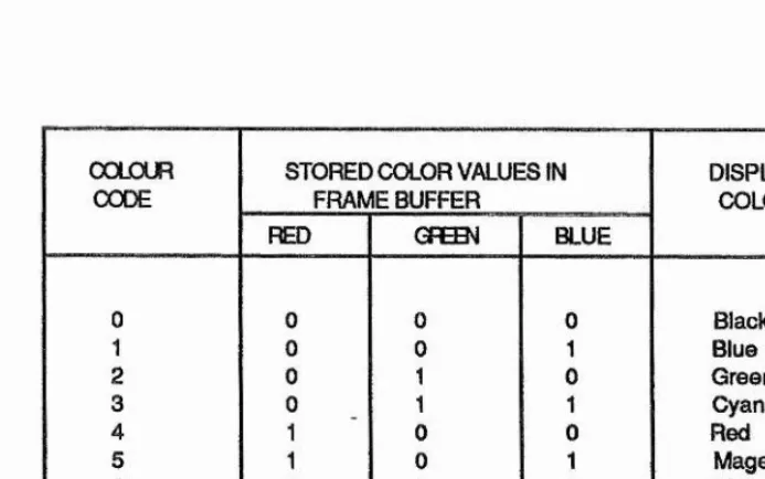
The simple run length encoding scheme can easily be extended to Include color. For color, the intensity of each of the red, green, and blue color

guns is given followed by the number of successive pixels for that color e.g..

Red Intensity Green Intensity Blue Intensity Run Length

Usually the color intensities are combined into a single integer, referred as color code, using a fixed number of bits. A simple scheme for storing color

code selections in the frame buffer of a raster system is shown in Figure 1-2.2. When a particular color code is specified in an application

program, the corresponding binary value is stored in the frame buffer for each

component pixel in the output primitives to be displayed in that color. The scheme is given in figure 1-2.2 allows eight color choices with 3 bits per pixel of storage. Each of the three bit positions is used to control the

intensity level (either on or off) of the corresponding electron gun in an RGB

monitor. The leftmost bit controls the red gun, the middle bit controls the green gun, and the rightmost bit controls the blue gun. Adding more bits per pixels to the frame buffer increases the number of color choices.

Run length coding can often substantially reduce the amount of memory needed to store images. Its advantage is maximised, in cases where the

images are made up of a few long runs. To produce long run lengths, very much

INTENSITY STORED INTENSITY VALUES DISPLAYED

CODES IN THE FRAME BUFFER GRAY

( Binary Code ) SCALE

0.0 0 (00) Black

0.33 1 (01) Dark Gray

0.67 2 (10) Light Gray

1.0 3 (11) White

Figure 1-2.1

Conversion of intensity values to integer codes for storage in a frame buffer accommodating a gray scale with four levels. Two bits of storage for each pixel position are needed in the frame buffer.

COLOUR

CODE STORED COLOR VALUES INFRAMEBUFFER DISPLAYEDCOLOR

RED GFB3^ BLUE

0 0 0 0 Black

1 0 0 1 Blue

2 0 1 0 Green

3 0 1 1 Cyan

4 1 0 0 Red

5 1 0 1 Magenta

6 1 1 0 Yellow

7 1 1 1 White

Figure 1-2.2

CHAPTER 1 REPRESENTATfON & EXACT COMPRESSION OF DIGITAL IMAGES.

Run length encoding can further be divided into two classes which are,

i. Linear scans.

ii. Space filling curves.

1-2.1 Linear Scan I Netravali and Haskell(1988)];

Linear scanning converts the two dimensional image intensity into a one dimensional waveform. The image is segmented into Ly adjacent horizontal

lines, and the image is scanned one line at a time, sequentially, left to right, and top to bottom with fly back at the end of each scanline, see Figure 1-2.3. It is

one dimensional in nature and takes advantage of the correlation between adjacent pixels on the scanline. For example, in a flying spot scanner a small spot of light scans across a photograph, and the reflected energy at any given position is a measure of the intensity at that point.

Figure 1-2.3

— —— Beamon.

CHAPTER 1 REPRESENTATION & EXACT COMPRESSION OF DIGITAL IMAGES.

1-2.2 Space Filling Curve :

Giuseppe Peano(1890) Introduced the idea of a space filling curve in the sense of a continuous mapping of the line segment (0,1) onto the unit

square and was closely followed by Hilbert(1891) and Sierpinski(1912). Peano, introduced the idea of space filling curves rather than polygons and

Hilbert and others introduced the idea of limiting sequences of polygons leading to space filling curves.

Peano showed how to produce a curve by moving a single point continuously over a square, such that it passes at least once through every point on the square and its boundary. The curve produced was indeed

continuous but it was impossible to draw unique tangents, since it is

impossible to specify the direction in which a points is moving. Two interesting points about the Peano curve were :

1) Its path seems to be one dimensional, yet at the limit it occupies a

two dimensional area.

2) It is a continous curve, but has no derivative.

Peano based his definition of space filling curve on a base three

representation of the points on the real line interval [0,1] and the points (x,y)

of the square 0 <= x <= 1 , 0 <= y <= 1. Essentially, a point of the above

interval was split into two real base three numbers by taking all the odd indexed digits in their sequential order for the value of x and all the even

CHAPTER 1 REPRESENTATION & EXACT COMPRESSION OF DIGITAL IMAGES.

are equally valid representations, was dealt with in a more complex manner, which need not be discussed in this report.

Hilbert generated a Peano curve with two end points, in other words,

Hilbert derived an alternative method of defining a space filling curve as the limit of polygons enclosed in the unit square, using a fourfold repetition of successive polygons which corresponded to a base two number representation,

as shown in Figure 1-2.5. At the limit Hilbert curve starts at the bottom left and finishes at the top left. A similar result based on the Peano technique was given by Moore(1900) to obtain a limiting polygon based on ninefold

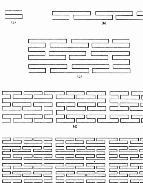
repetitions of successive polygons. These polygons are known as Peano

Polygons. The first three Peano polygons P1,P2,P3 are shown in Figure 1-2.4.

The three steps of the illustration show how Waclaw Sierpinski

generated a closed Peano curve (see Figure 1-2.6a). Sierpinski polygons differ from Hilbert and Peano polygons. The principal difference as Wirth[1976] pointed out is that Sierpinski curves are closed curves made up of four parts,

which are connected by the four straight lines in the outermost four corners. Cole(1983) showed that S^' can be obtained from S n -i' by suitably rotating and shifting 8 ^-1 ' to four new positions and joining them by three lines. S y , S2', S3' are shown in the Figure 1-2.6b. Further S3 (see Figure 1-2.6a) is

obtained by rotating S3' (see Figure 1.2.6b)four times and finally closing the

last gap. Wirth suggested that Sq is a square standing on one corner. It means

the starting curve is the single point [1,0]. Recursive algorithms for drawing

these and other space filling curves have been given by Wirth(1976),

Goldschlager(1981) and Witten and Wyvill (1983). Griffiths(1985) discusses table driven algorithms for generating space filling curves.

Helge Von Koch[Gardner(1967)], proposed in 1904 another curve which

r—' s r—'

*~ i H

Figure 1-2.4. Peano polygons.

(a)

(

S\

sv

(b)

CHAPTER 1 REPRESENTATION & EXACT COMPRESSION OF DIGITAL IMAGES.

in length. Like a Peano curve its points have no unique tangent, i.e., continous

but no derivative. The first four orders of Helge Von Koch's snow flake are illustrated in Figure 1-2.7.

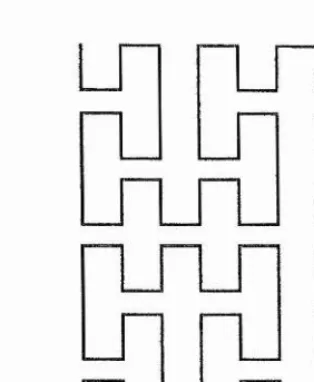
Griffith(1986) investigated space filling curves and described a method for generating new ones. He considers the space filling curve in the unit square defined as the limit of a sequence s*j,S2 of continuous curves

which pass through every point of the square. This can be viewed as a

tessellation of square tiles all of which have the same pattern but with the orientation of the pattern varying. Firstly a tile has an n x n grid marked on it and the centres of each grid-square are taken as permissible points for the

construction of a continuous open path that does not intersect. The resulting path must have endpoints such that n2 tiles can be fitted together and the

individual paths joined up with standard steps as shown in Figure 1-2.8. Griffiths at this stage had shown how to generate new space filling curves which would traverse squares.

Cole(1983) has shown how Peano, Hilbert and Sierpinski polygons can all be obtained recursively from a single point. Cole showed explicit mappings

between the first n non-negative integers and the n sequentially traversed vertices of any of the Peano polygons and also a generalisation of these polygons. Such polygons have been called murray polygons since they are derived using multiple radix or murray arithmetic. A formal definition and

more detailed discussion of murray polygons will be given in the following chapters.

The advantages of using space filling polygons for this purpose arise from the fact that in general the curve passes through a lot of points local to

Figure 1-2.7. The first four orders of Helge von Koch's snowflake (Martin[6?]).

nmim

CHAPTER 1 REPRESENTATION & EXACT COMPRESSION OF DIGITAL IMAGES.

each other in two dimensions. This pixel coherence can be exploited in many areas of image processing. This we will see in the following chapters.

Moreover the Hilbert polygons include quadtree scanning as a particular, case with no additional computation or complex data structures required to record or to scan them.

1 3 Quadtree Encoding :

The term quadtree is used to describe a class of hierarchical data

structures whose common property is that they are based on the principle of recursive decomposition of space. They can be differentiated on the following bases :

1. the type of data that they are used to represent,

2. the principle guiding the decomposition process,

3. the resolution ( variable or not ).

Quadtree representation can be used for point data, regions, curves, surfaces, and volumes.The decomposition may be into equal parts on each level

(i.e., regular polygons and termed a regular decomposition ), or it may be governed by the input. The resolution of the decomposition (i.e. the number of times that the decomposition process is applied ) may be fixed, or it may be governed by properties of the input data.

Quadtrees are generated by successively dividing a two dimensional region into quadrants. Each node in the quadtree has four data elements, one for each of the quadrants in the region as Illustrated in Figure 1-3.1. If all

Quadrant

0

Quadrant

1

Quadrant 3

Quadrant 4

0 1 2 3

Figure 1-3.1

Region of a two dimensional space divided into numbered quadrants and the associated quadtree node with four data elements.

0 1

3 --- - 2

---Region of a Two-Dimensional

space

0 1 2 3

0 1 2 3

Quadtree Representation

Figure 1-3.2

CHAPTER 1 REPRESENTATION & EXACT COMPRESSION OF DIGITAL IMAGES.

set in the data element to indicate that the quadrant is homgeneous. Suppose

all pixels in quadrant 2 of Figure 1-3.1 are found to be red. The color code for red is then placed in data element 2 of the node. Otherwise the quadrant is said to be heterogenous, and that quadrant is itself divided into quadrants (see Figure 1-3.2). The corresponding data element in the node now flags the quadrant as heterogeneous and stores the pointer to the next node in the

quadtree. For a heterogeneous region of space, the successive subdivisions into quadrants continues until all quadrants are homogeneous. Figure 1-3.3 shows a quadtree representation for a region containing one area with a solid color that is different from the uniform color specified for all other areas in the region.

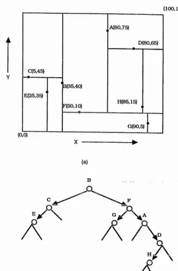
Finkel and Bentley(1974) proposed another definition for a quadtree. Here space is partitioned into rectangular quadrants. It is primarily used to

represent multidimensional point data and can be referred as a point quadtree. In two dimensions each data point is a node in a tree having four sons. These four sons corresponds to a quadrant labeled in order NW, NE, SW, and SE. The desired record is searched on the basis of its x and y coordinates. At each node of the tree a four way comparison operation is performed and the appropriate

subtree is chosen for the next test. Reaching the bottom of the tree without finding the record means that the record which we are looking at is not present in the quadtree and it can now be Inserted at this position. The shape of the resulting tree depends on the order in which records are Inserted into

it. A point quadtree is illustrated in Figure 1-3.4.

Point quadtree are useful in applications that involve search. They can also, be used to solve a measure problem like determination of all records

within a specified distance of a given record. Search operations using point

quadtrees are given in details by Bentley and Stanat(1975). Point quadtrees

0 0 0 0 0 0 0 0

0 0 0 0 0 0 0 0

0 0 0 0 1 1 1 1

0 0 0 0 1 1 1 1

0 0 0 1 1 1 1 1

0 0 1 1 1 1 1 1

0 0 1 1 1 1 0 0

0 0 1 1 1 0 0 0

(a) _(b)

o # e #

37 38 39 40 57 58 59 60O

(d)

F Ig u rel - 3 . 3 . A region, its binary array, its maximal blocks, and the corresponding quadtree. (a) Region.

(b) Binary array.

CHAPTER 1 REPRESENTATION & EXACT COMPRESSION OF DIGITAL IMAGES.

are useful with two dimensional space. As cited by Samet(1984), the problem with a large number of dimensions is that the branching factor becomes very

large (i.e., 2^ for k dimensions). The storage for each node as well as for many NIL pointers for terminal nodes increases. Bentley(1975) proposed W tree,

which is an improvement on the point quadtree. It avoids the large branching factors. It is a binary search tree with the distinction that at each level of the tree a different coordinate is tested when determining the direction in which a branch is to be made. In the case of two dimensions (i.e., a 2-d tree), the

x-coordinates will be compared at the root and at even levels, whereas the y -coordinates are compared at odd levels. The root is assumed to be at level zero. Each node has two sons. A k-d tree corresponding to the point tree of

Figure 1-3.4 is given in Figure 1-3.5.

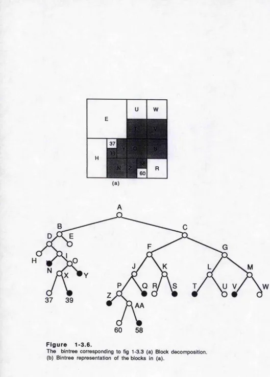
An alternative tree structure that uses. an analogy to the k-d tree given by Bentely(1975) is the bintree proposed by Samet and Tamminen(1984). Here, the space is always subdived into two equal-sized parts alternating between the X and the y axes. The advantage is that a node requires space only for pointers to its two sons instead of four sons. In addition, its use generally

leads to fewer leaf nodes. While dealing with higher dimensional data ( e.g., three dimensions) less space is wasted on NIL pointers for terminal nodes. A bintree is Illustrated in Figure 1-3.6.

The problem with the tree representation of a quadtree is that it has a cosiderable amount of overhead associated with it. Moreover each node requires additional space for the pointer to its sons. This is a problem with large images that cannot fit into core memory. Consequently, there has been a

considerable amount of interest in pointerless quadtree representations. They

(100,100)

A(60,75)

A

C(5,45)

8(35,40)

H(85,15]

G(90,5)

(0,0)

(a)

E

A A A

(b)

Figure 1-3.4

(100,100)

A(60,75)

A

C(5,45) Y

B(35,40) E(25,35)

H(85,15) F(50.10)

G(90,5) (0,0)

X ”

(a)

(b)

Figure 1-3.5.

60

58

Figure 1-3.6.

CHAPTER 1 REPRESENTATION & EXACT COMPRESSION OF DIGITAL IMAGES.

can be grouped into two categories.

i. Collection of leaf nodes.

ii Traversal of the nodes of its quadtree.

1-3.1 Leaf node :

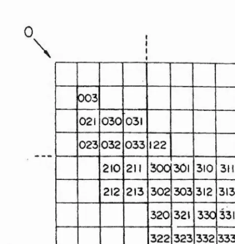
In the leaf node category, each leaf or pixel is encoded in a weighted quatenary code, i.e., with digit 0, 1 , 2 , 3 in base 4, where each successive

digit represents the quadrant subdivision from which it originates. The NW

quadrant is encoded with 0, the NE quadrant with 1, the SW with 2, and the SE with 3. For example, if a pixel or leaf Is encoded as 321, this means that pixel

or leaf belongs to the SE quadrant in the first subdivision, to the SW quadrant in the. second and the NE in the third (final) subdivision (see Figure 1-3.7).

While encoding an image as a collection of leaf nodes, there is no need to include the locational code for every leaf node. Gargantini (1982) only

retains the locational codes of the BLACK nodes and terms the resulting representation a linear quadtree. The codes for WHITE blocks can be obtained by using the ordering imposed by the sort without reconstructing the

quadtree. All arithmetic operations on the locational code are performed by

using base 4 numbers as explained above. An additional code, as a don't care, is used by Gargantini(1982), Klinger and Dyer(1976), Abel and Smith (1983), Oliver and Wiseman(1983) to yield an encoding where each leaf in a 2^i by 2^ image is n digits long. A leaf corresponding to a 2^ by 2^ block (k<n) will have n - k don’t care digits. Once all the black pixels are encoded into their corresponding quaternary codes, then they are sorted and stored in an array or

list. If four pixels have the same representation except for the last digit, they are eliminated from the list and are replaced with a code of (n-1) quaternary

0

\

/

/

003

021 030 031 023 032 033 122

210 211 300 301 310 311

212 213 302 303 312 313 320 321 330 331 322 323 332 333

\

CHAPTER 1 REPRESENTATION & EXACT COMPRESSION OF DIGITAL IMAGES.

digits followed by some kind of marker ( don't care ), here denoted by X. For instance, if pixels 310, 311, 312, and 313 are all in the array, they can be replaced by 3 IX . Similarly, 30X, 31X, 32X, 33X can be replaced by 3XX and so forth, where X is the don't care digit greater than 3. Such an encoding has the

interesting property that when the codes of the nodes are sorted in increasing order, the resulting sequence is the postorder traversal of the blocks of the

quadtree. The main advantages of linear quadtrees, with respect to quadtrees are:

i Space and time complexity depend only on the number of black nodes.

ii. Pointers are eliminated.

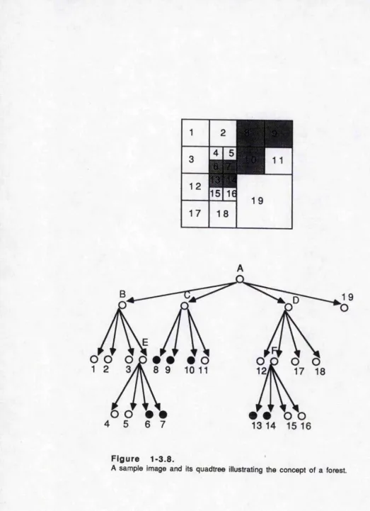
Jones and lyenger(1984) and Raman and lyenger(1983) introduced the concept of a forest of quadtrees that is a decomposition of a quadtree into a collection of subquadtrees, each of which corresponds to the maximal square. The maximal square is identified by refining the concept of a nonterminal node

to indicate some information about its subtrees. An internal node is said to be of type GB if at least two of its sons are BLACK otherwise the node is said to be of type GW.For example, in Figure 1-3.8 ,nodes 0,

E,

nodes A, B, and D are of type GW. Each BLACK node with a label of GB is said to be a maximal square. A forest is the set of maximal squares that are not

contained In other maximal squares and that span the BLACK area of the image. The forest corresponding to Figure 1-3.8 is { C,E,F}. The elements of the forest

are identified by base 4 locational codes. For the path code or locational code the scheme is the same as defined by Gargantini. This type of representation can save space since W HITE items are ignored.

o o

17

18

10

11

# e o o

13

14

15

16

Figure 1-3.8.

CHAPTER 1 REPRESENTATION & EXACT COMPRESSION OF DIGITAL IMAGES.

A linear hierarchical quadtree (LHQT) ( Unnikrishnan, Venkatesh, And

Shankar{1987)) is a modified version of a linear quadtree[Gargantini(1982)J. Since the level of the hierarchy indicates the size of the black nodes, the additional code, don't care which was used by Gargantini can be deleted. As a

consequence, the quadtree code at level k will contain (n-k) digits only.

Unnikrishnan called these modified codes the Linear Hierarchical Q-codes

(LHQC). The set of all the n arrays of LHQC Is called the Linear Hierarchical Quadtree(LHQT). For example, if a leaf has code 3XX, where X >= 3 , then all the additional digits i.e., X can be replaced to give a new code which will now be equal to 3 (see Table 1-1).

Level

Hierarchically

ordered q-code q-codes ( LHQC )Linear hierarchical

2 244 2

1 124 12

134 13

0 300 300

301 301

302 302

320 320

322 322

Table 1-1. The LHQT for an arbitrary binary Image, (4 Is the additional digit representing X).

Anedda and Felician(1988) suggested a new compression technique,

referred to as P-compression. Here a pixel code be divided into a prefix of P digits, 1 <= P < n, and a suffix of (n-P) digits. Every pixel belonging to the quadrant originated by the first P quadrant subdivisions that Is consequently

of size 2(n-P) pixels has the same prefix. Then store all distinct prefixes once; each of them will be followed by the number of pixels having that

prefix,

CHAPTER 1 REPRESENTATION & EXACT COMPRESSION OF DIGITAL IMAGES.

and by the corresponding suffixes (see Figure 1-3.9a). They have compared the

results with those obtained by Gargantini(Linear-quadtree). Two cases namely the best case and the worst case, are considered (see Figure 1-3.9 a,b, and c

). In the best case Gargantini's compression algorithm is shown to be more efficient than P-compression, since the quadtree compression consists of a

single pixel code with m don't care digits( where m is the size of a quadrant), in its rightmost positions, whereas a P-com pressed quadtree needs more

codes, that is more storage space.lt has been pointed out that in the worst case P-compression is better if m<=4.

1-3.2 Traversal of the nodes of its quadtree :

The second pointerless representation Is in the form of a preorder tree traversal ( i.e., depth first ) of the nodes of the quadtree. The result is a string consisting of the symbol "(" , "B", "W" corresponding to GRAY (i.e., if all pixels within a quadrant are not of same color), BLACK, and WHITE nodes respectively. This representation is due to Kawaguchi and Endo (1980) and is

called DF-expression. For Example, the Image of Figure 1-3.3 has

(W(WWBB(W(WBBBWB(BB(BB(BBBWW as its DF-expression (assuming that sons are traversed In the order NW, NE, SW,SE). The original image can be

reconstructed from the DF-expression by observing that the degree of each nonterminal I.e., GRAY node is always 4.

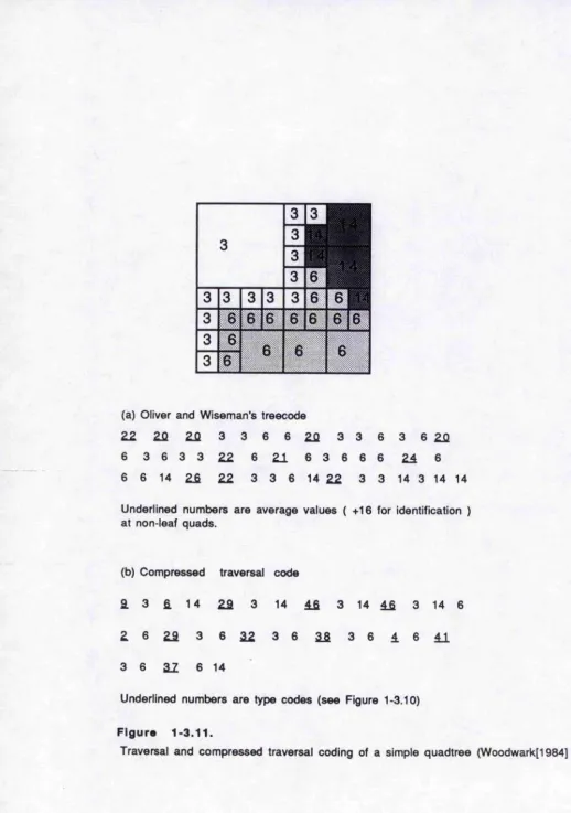
Oliver and Wiseman(1983) also reported a linear code which specifies a quadtree in depth first order. Their data Items consist of five-bit numbers,

of which the last four bits constitute the color value. If leaf, color the square with value in 4 bit field, otherwise the color value refers to an average of the

quads beneath. Figure 1-3.11(a) illustrates a simple quadtree in their

encoding. In the above coding, the value which indicates a non-leaf quad is

Linear Quadtree P-Compressed Quadtree

003230020 0032300

003230022 5

003230023 20

003230031 22

003230031 23

003230033 31

33

(a)

(b) (c)

Flgure1-3.9.

(a) P-compression coding to a linear quadtree

(b) Best case position of a 2 by 2 ^ region in a 2 ^ by 2 " binary image.

CHAPTER 1 REPRESENTATION & EXACT COMPRESSION OF DIGITAL IMAGES.

repeated many times. The compressed quadtree scheme was designed by Woodwark(1984) in order to obtain the compression of the node list resulting from a depth-first visit of the quadtree. This method consists in associating a type code with each non-terminal node in the tree. There are 52 possible type

codes for the sons of any non-leaf quadrant { see Figure 1-3.10 ). These allow for any or all of the sons of that quadrant to be defined further down the tree. If, for example a non-leaf quadrant has dependent leaf of two colors, A and B,

the record of representing that quadrant will consist of the appropriate type code, followed by the color values of A and B in the order defined by the type code. Any dependent non-leaf quadrants will follow in traversal order.

Figure 1-3.11(b) shows a simple quadtree represented using this compressed traversal code.

The quadtree is proposed as a representation for binary images

because its hierarchical nature facilitates the performance of a large number

of operations. Most images are traditionally represented by structures such as binary arrays, raster(i.e, run length), chain code(i.e., boundaries) or

polygons(vectors), some of which are chosen for hardware reasons ( e.g., run

lengths are particularly useful for rasterlike devices such as television) . Conversion from these methods to quadtrees is given in Samet(1984,1981b), Unnikrishnan, and Venkatesh(1984).

1-4 Volume Data

Extension of the quadtree to represent three-dimensional objects by use of octrees has been proposed independently by many researchers

Hunter(1978); Jaclins and Tanimoto(1980); Meagher(1982); Reddy and Rubin(1978) as cited by Samet(1984). The process begins with a

2n by 2n by 2n object array of unit cubes or voxels( volume elements)

No leaf quad*

One cdouf of leaf quad ___ ____ ___

3E3S3S3!aSèlS

1 jCZSSDlâiij_{) u » .«>}

Two coiou's of leaf quad

Three tofou** of leaf quad

four cofourt of leaf quad

[Â1 jH ) f n fP | it 0 M # «raw ti

£ 7 \ lOkefw «•d-ImT « W * e n !' iy{m fcOEw W P n

Arevertcl

(a) Oliver and Wiseman's treecode

22 2Û 2Û 3 3 6 6 2 Û 3 3 6 3 6 22

6 3 6 3 3 2 2 6 2 1 6 3 6 6 6 24 6

6 6 14 26 22 3 3 6 14 2 2 3 3 14 3 14 14

Underlined numbers are average values ( +16 for identification ) at non-leaf quads.

(b) Compressed traversal code

a 3 fi. 14 2 a 3 14 4LB 3 14 42 3 14 6

2 6 2 2 3 6 22 3 6 22 3 6 1 6 4 J.

3 6 2 1 6 14

Underlined numbers are type codes (see Figure 1-3.10)

Figure 1-3.11.

CHAPTER 1 REPRESENTATION & EXACT COMPRESSION OF DIGITAL IMAGES.

[Jaclins and Tanimoto(1980)] (also termed as obels [ Meagher(1982)]. The octree is an approach to object representation similar to the quadtree, and is based on the successive subdivision of an object array into octants. If the

array does not consist entirely of Ts or entirely of O’s, then it is subdivided into octants, suboctants, etc. until cubes (possibly single voxels) are obtained that consist of Ts or O’s; that Is they are entirely contained In the region or entirely disjoint from it. This process is represented by a tree of out degree 8

in which the root node represents the entire object with octants labelled as in Figure 1-4.1, and the leaf nodes are said to be BLACK or WHITE , depending on whether their corresponding cubes are entirely within or outside of the

object, respectively. All nonleaf nodes are said to be GRAY. Figure 1-4.2 contains an example object in the form of a staircase and its corresponding octree. The labels denote the octant numbers associated with each son by

using the labelling convention of Figure 1-4.2.

Many of the algorithms obtained for the quadtree, can be extended to the octree. Gargantini(1983) makes use of a pointerless representation termed a linear octree ( analogous to the linear quadtree, Gargantini(1982). He

represented each pixel by an octal integer in a weighted system. Thus the

digits of weight l <= h <= n identifies the largest octant to which the pixels belong at the hfh subdivision, in the planar case, a quadrant is

subdivided into four squares identified by NW ,NE,SW and SE. An additional notation “Forward" and "Backward" ( F and B ) has been introduced to

distinguish between the four cubes nearer to the viewer with respect to the

other four cubes. Here octant NWF is encoded with 0, octant NEF with 1, octant SW F with 2, octant SEF with 3, octant NWB with 4, octant NEB with 5, octant SWB with 6, and in the last octant SEB with 7.

Region of a Three-Dimensional Space

0 1 2 3 4 5 6 7

Data Elements in the Representative Octree Node

Figure 1-4.1.

Region of a three-dimensional space divided into numbered octants and the associated octree node with eight data elements (octant 3 is not visible) .

0 1 2 3

(b)

Figure 1-4.2.

Example object (a) and its octree (b).

0 = BLACK = "Full";

□ = WHITE = "VOID" (empty);

CHAPTER 1 REPRESENTATION & EXACT COMPRESSION OF DIGITAL IMAGES.

Figure 1-4.3

Representation of an object with n=2.

Once all the black pixels are encoded, condensation can be applied as discussed in Gargantini(1982) i.e., the representation for the region shaded in

Figure 1-4.3(Gargantini(1983).

{ 01,10,11 ,12 ,13 ,14 ,15 ,16 ,17 ,35 ,5 1}

will be replaced by,

{01,1X ,35.51}

where X is the marker or don't care digit defined earlier, with an integer>7.

CHAPTER 1 REPRESENTATION & EXACT COMPRESSION OF DIGITAL IMAGES.

All the algorithms, explained above for octrees, have a common disadvantage. The entire three-dimensional image array must be loaded into computer memory from the start and left there throughout a session.

Yau and Srihari(1983), proposed a general approach to construct a

2d-tree (or hyperoctree), representing a d-dimensional binary image from the

2^ -1-trees representing (d-l)-dimensional cross sections ( or slices) of the

image, orthogonal to any of the axes. The word hyperoctree is defined by

Yau and Srihari, for a d-dimensional binary image. Here a d-dimensional image is recursively divided into 2^ hyperoctants giving a 2d-tree or hyperoctree.

Since the work given in this thesis is based on two-dimensional and

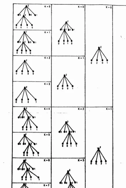
three-dimensional Images, we need not discuss d-dimensional images in this report. The quadtree to octree conversion algorithm developed by Yau and Srihari is established in such a way that 2^ quadtrees qo»qi» <^2*^-1, of

which are generated from the array of side 2^, are sequentially loaded. Then q i is merged with qg, qg is merged with ...,q2 0-i with q2n_2, to give 20-1 new trees

q'o»q'i

we obtain the octree. The only operation at every merging is to copy the

subtree whose root is at a certain depth onto the corresponding node of the other tree while traversing the two trees in parallel, this is explained in

Figure 1-4.4. Just to explain the theory discussed above, we consider eight quadtrees, whose origin is not known. For more details see Xiaoyang, Tosiyasu ,Fujishiro, and Noma(1987) and Chien and Aggarwal(1986), and Shrhari(1981).

K « 0

0 0 ( 0

K « 1

0 0 1 0

A

K-2

A

K » 3

K « 4

0 0 1 1

K = S

0 # 1 1

K -t

# 1 1

K-7

1 0 1 0

K " 0

0 0 1 0

K - 1

A

K"2

0 0 1 1

K -3

§ @ 1 1

K . 0

A

K«1

Â

Chapter 2

2 . M URRAY POLYGONS 2 0

2 - 1 Introdution 2 0

2 - 2 Murray Polygons 20

Gray Codes or Cyclic Progressive Numbers 2 3

Direct Peano Transformations 2 5

Murray Arithmetic 2 6

Murray Transformation 2 8

Mixed Scan 3 1

Some Lemmas 3 2

Implementation Of Murray Scan 3 9

Original Implementation 3 9

A Faster Murray Scan Algorithm 4 2

Hardware Implementation 4 6

Three-Dimensional Cartesian Coordinates 4 6

Extension To 3-D And n-D Murray Polygons 4 7

Method One 4 7

Some Lemmas 5 0

Second Method 6 2

Polar Murray Scan 5 4

Polar Coordinates 5 4

Changing Coordinates Systems 5 5

Graphs In Polar Coordinates 5 6

3D And Higher Dimensional Polar Coordinates 5 6

Cylindrical And Spherical Coordinates 5 6

Implementation Cf Planar Polar Murray Scan 5 9

Cylindrical Polar Murray Scan 6 1

Spherical Polar Murray Scan 6 1

2-2.11 Application Areas 62

Scanning 6 2