Remote sensing tools for the objective quantification of tree structural condition from individual trees to landscape scale assessment

(1)

Remote Sensing Tools for the

Objective Quantification of Tree

Structural Condition

from Individual Trees to Landscape

Scale Assessment

Jon Murray

This thesis is submitted for the degree of

Doctor of Philosophy

October 2018

Lancaster Environment Centre

(2)

(3)

(4)

“The importance of the forest canopy to forestry and forest research has been reflected in the ingenuity of foresters in devising methods and instruments to measure it.”

(5)

This thesis has not been submitted in support of an application for another degree at this or any other university. It is the result of my own work and includes nothing that is the outcome of work done in collaboration except where specifically indicated. Many of the ideas in this thesis were the product of discussion with my supervisory team; Prof. Alan Blackburn, Dr. Duncan Whyatt and Dr. Chris Edwards.

Excerpts of this thesis have been published to the following academic publications:

Murray, J., G.A. Blackburn, J.D. Whyatt and C. Edwards (2018). "Using Fractal Analysis of Crown Images to Measure the Structural Condition of Trees." Forestry: An International Journal of Forest Research 91(4): 480-491.

Murray, J., Gullick, D., Blackburn, G. A., Whyatt, J. D., & Edwards, C. (2019). ARBOR: A new framework for assessing the accuracy of individual tree crown delineation from remotely-sensed data. Remote Sensing of Environment, 231, 111256.

Jon Murray

(6)

Tree management is the practice of protecting and caring for trees for sustainable, defined objectives. However, there are often conflicts between maintaining trees and the obligation to protect targets, such as people or infrastructure, from the risks associated with the failure of trees and major limbs. Where there are targets worthy of protection, tree structural condition is typically monitored relative to the prescribed management objectives. Traditionally, field methods for capturing data on tree structural condition are manual with a tree surveyor taking very limited direct measurements, and only from parts of the tree that are within reach from the ground. Consequently, large sections of the tree remain unmeasured due to the logistical complications of accessing the aerial structure. Therefore, the surveyor estimates tree part sizes, approximates counts of relevant tree features and uses personal interpretation to infer the significance of the observations. These techniques are temporally and logistically demanding, and largely subjective.

(7)

delineation algorithms. The framework is then used to identify an optimal ITC delineation algorithm which is applied to aerial laser scanning data to map individual trees and extract a point cloud for each tree. Metrics are then derived from the point cloud to classify a tree according to its structural condition, a process which is then applied to the tree population across an entire landscape. This provides information with which to spatially optimise tree survey and management resources, improve the decision making process and move towards proactive tree management.

(8)

Acknowledgements

There are always many people to thank for their individual help during the course of a project like this, too many to name everyone individually, but I extend genuine gratitude to all those who have helped me on this journey. Especially to all the office dwellers of B31a, and in particular to Miss B for, you know, absolutely everything! Hopefully, these brief words will go some small way in conveying my appreciation to everyone who has helped over the years.

To my supervisors Alan, Duncan and Chris, I am of course, so very grateful for all the help and insight you have provided over the years. In particular during difficult times where your support and guidance was most needed, and was freely given. Thank you all.

To Vassil, my thanks for the many hours of help with the fieldwork, always with a genuine interest and willingness to shoulder whatever task (and equipment!) you could.

A special thanks to Mr. Oswald Copperpot for the many hours spent surveying in the woods and never complaining or wanting to go home early, no matter how grotty the days were! Sadly, you passed before seeing me get to the end of this but I know I couldn’t have got here without your company and friendship along the way.

(9)

irreplaceable family time. I can’t make any of that lost time back, but I promise you

that things will be better now this PhD is finally finished!

Finally, to Sue. Although it has turned out not to have been the journey that we originally hoped for, I offer you my thanks for all your support which ultimately helped me to reach the end, and to finish this ‘little job’.

(10)

List of Tables

Table 1 An overview of tree surveying methods currently in use in the forestry, arboriculture or tree management sectors. The word ‘objective’ refers to direct measurement or factually acquired data. The word ‘subjective’ refers to instances

where a field operative uses interpretation, estimates or best guess methods to acquire ‘measurements’ for the survey method. This list is not exhaustive, but is

representative of tree surveying methods frequently used in the UK, USA and worldwide. ... 10 Table 2 Categories of manual tree measurements taken during field capture of

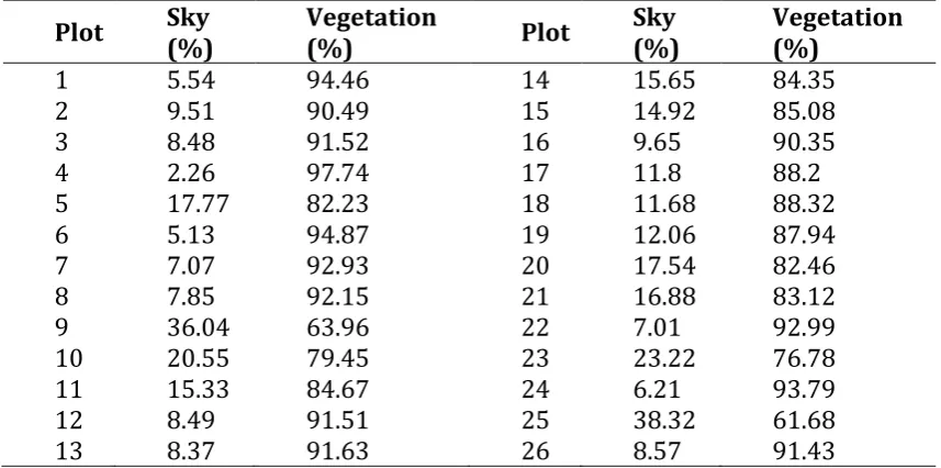
ground reference data. Examples of the data recorded are also shown. ... 54 Table 3 Calculation of vegetation cover at 26 survey plots. Images were captured at

each location and amount of sky or vegetation that occupies the image was calculated using CAN_EYE. ... 57 Table 4 Summary record of ground reference field and research sites used within a

remote sensing investigation, and the number of trees for the types of data recorded at each location. ... 63 Table 5 LiDAR data types and description provided in ASCII format for LiDAR

flightlines over Eaves Wood, UK. ... 65 Table 6 Descriptions of analytical metrics used in an investigation to quantify tree

structural condition. ... 81 Table 7 Threshold limits of tree condition categories, expressed in fractal

dimensions (Df). ... 87 Table 8 A meta-study of several match-pairing methods showing the base matching

(14)

Table 9 Introduction of data noise following modification of the normal distribution and standard deviation (SD) effect on the data population relative to data noise levels. ………...115 Table 10 Quantification of ARBOR framework scores for four individual tree crown

(ITC) delineation techniques, when compared to known tree location, height and crown areas of ground reference tree data. ... 125 Table 11 LiDAR pulses returned for a combination of six flight line passes of Eaves

Wood, Lancashire, UK. Point data 1 is unconsolidated results of all flightlines, while point data 2 is an optimised area of overlapping flightlines. ... 139 Table 12 Standardized and raw discriminant function coefficients as unstandardized

regression weights for LiDAR return (r) variables (Murray, Blackburn et al. 2014) ………...142

Table 13 Correlations between the dependent (return (r)) and canonical variables (Murray, Blackburn et al. 2014)... 142 Table 14 Description of measurements calculated from LiDAR point cloud data,

grouped into themed areas of inventory, intensity, area, height and other. Adapted from Parkan (2018) ... 146

Table 15 Description of a range of classifier models used in assessing the accuracy of trained models in a supervised learning analysis. ... 147 Table 16 Chi-square (χ2) validation of two classification models (medium kNN and

RUS Boost) that were trained using different training data populations (N=100 and N=235). ... 157 Table 17 A cross tabulation validation results of a ground reference dataset (GRD) that

(15)

(16)

List of Figures

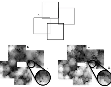
Figure 1 A visualisation of CHM’s from LiDAR data, using two different techniques. a. The outline of four woodland survey plots. b. typical pixelated CHM as used in many RS studies, with data pitting that causes analysis errors (Ben-Arie, Hay et al. 2009) (circular inset i, poor tree canopy resemblance with data pits as black pixels). c. a novel “splatted” CHM, closely resembling tree canopies, with data pits

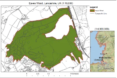
eliminated (Khosravipour, Skidmore et al. 2016) (circular inset ii., tree-like canopy edge with no data pits). The four conjoined square shapes are four separate field survey plots, with each plot measuring 20x20 metres (400m2_{) on the ground. ... 36} Figure 2 The approximate location of Eaves Wood, Silverdale, Lancashire, UK. ... 52 Figure 3 Equipment required for taking beneath crown hemispherical photographs for

use in crown structure analysis 1. dSLR camera with a hemispherical lens adapter, compass and level 2. Standard camera tripod, 3. Surveyors measuring tape, 4. GPS/data logger, 5. Tree survey data sheets, 6. Sunnto clinometer, 7. DBH tape (not shown). ... 55 Figure 4 Geolocation of ground control points (a), and undertaking a first order

triangulation survey (b), to locate survey plots within woodland to aid data processing in an investigation gathering LiDAR data of Eaves Wood, Silverdale, Lancashire, UK. ... 59 Figure 5 A survey plot layout for capturing data in an ALS LiDAR investigation

(17)

Figure 6 An assessment of structural diversity of a tree population in Eaves Wood, Lancashire, UK. The data follows an ideal ‘reverse-J’ distribution, which indicates

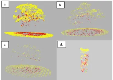
a structurally complex and diverse population (Kerr, Mason et al. 2002). ... 62 Figure 7 Individual trees delineated from ALS LiDAR data of Eaves Wood. a) a tree

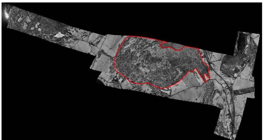
in good crown condition, b) a tree in moderate crown condition, c) a tree in poor crown condition, d) a monolith of a dead tree (no crown) and ground points removed for visual clarity. Return (r) pulses R1-3 can be seen as yellow, red and green respectively. ... 64 Figure 8 Intensity image of Eaves Wood, UK, with intensity values ranging from 0

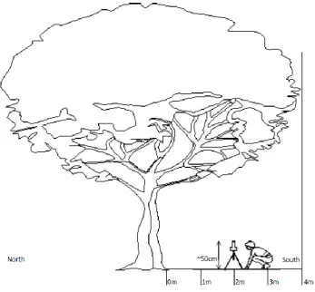
(dark) to 255 (white). The image also shows the boundary of Eaves Wood, outlined in red. ……….65 Figure 9 A schematic of the field method for taking a hemispherical picture from

beneath a tree canopy. The camera is situated on a standard tripod, and is levelled and pointing towards the zenith viewing point (90° from the horizontal elevation). In this example, the full extent of the crown is four metres along the southern axis, and the image is taken at the two metre mid-point. ... 73 Figure 10 Classification descriptors for the subjective arboricultural assessment of

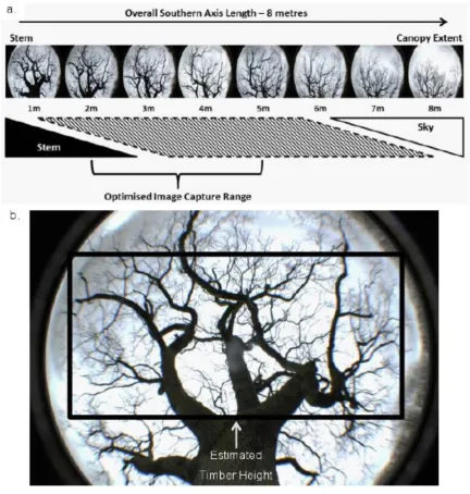
trees. Estimated Remaining Contribution (ERC) refers to a methodology used to consider the health, condition and structure of the tree and aids in classifying the tree in to the different categories adapted from (Barrell 1993, Lonsdale 1999, Barrell 2001, NTSG 2011, BSI 2012). Note: The images show trees in leaf-on condition to enable ease of comparison for the condition types. ... 75 Figure 11 A schematic showing the optimised range for image capture (a), and the

(18)

elements not required, are removed from the image by only analysing the structure inside a user selected bounding box area (b). The use of a bounding box allows images of both individual trees and trees within closed canopies to be analysed. . 78 Figure 12 A procedural workflow showing how tree structure images are processed for

the computation of image metrics ... 85 Figure 13 Sample subset of predictor variables used to define the characteristics of

different tree structures (n64). The annotations Good, Moderate, Poor and Dead refer to the field observed condition of the individual trees. Only with the measure of fractal dimension (a.), provides homogeneous clustering of field observed conditions as identified by the threshold lines. Not all predictor variables used in this study are visualised in this plot ... 89 Figure 14 A proportional odds model to indicate the probability (P) that tree structure

images, quantified in fractal dimensions (Df), are indicative of an observable tree structure condition and known reference standard (n64). Tree images were measured for structural complexity in Df. The box plot extents identify the P that the structures show characteristics of the reference standard. ... 90 Figure 15 Gaussian overlap used for measuring data agreement between two data sets,

where the difference between the two shapes is quantified using the Jaccard similarity coefficient. ... 108 Figure 16 500 synthetic trees representing ground reference (GR), and RS-derived

LiDAR datasets. a) models 500 GR trees, and b) represents RS-derived trees with increased noise and tree losses. This replicates typically observed effects in aerial LiDAR derived canopy height models. ... 114 Figure 17 An example of Gaussian curves demonstrating the change on data

(19)

intentionally introduces data noise to a remote sensing dataset of synthetic trees. ………...115

Figure 18 A combination of three data match-pairing methods being tested for the ability to achieve predicted data pairings between synthetic GR and RS-derived data. Each pixel in plots a-c represents an assessment of normalised root mean squared error (NRMSE) at differing levels of data noise and loss. Plots d-f represent the effect of the match-pairing on the data population, expressed as a pairing ratio. ... 118 Figure 19 A working example of the ARBOR framework workflow for the

quantification of match-pairing agreement between remote sensing derived and ground reference data. Notes: AMPS = averaged matched-pairing similarity index, DSS = dataset size similarity index ... 122 Figure 20 ARBOR scores comparing the match-pairing success between four

different ITC delineation techniques acquired from aerial LiDAR data with ground reference data over 26 survey plots. ... 124 Figure 21 Outline of Eaves Wood, Lancashire, showing locations of the transect line

and ground reference plots. The grey boxes indicate the overlapping LiDAR flightlines, while the black box identifies the flightline area that achieved 100% overlap, corresponding with the central transect and ground reference plots. ... 139 Figure 22 Tree canopies as drawn as circular shapes in ArcGIS at 1:125 scale. The

canopies are created with scaled measurements and orientated in the direction as they were found in data collection at Eaves Wood, Silverdale, Lancashire, UK. Also shown in the image is the transect line (red) and plot area (green) used in the investigation. ... 141 Figure 23 Subject trees in manually observed conditions: a, b, c, and d = good,

(20)

representations of trees scanned using DR ALS LiDAR, with pulse returns shown: r1 (Yellow), r2 (Red), r3 (Green). ... 143 Figure 24 ITC delineations of individual trees across the full study site flightline.

These unsurveyed trees will be classified using their biophysical characteristics as observed in ALS LiDAR data. ... 145 Figure 25 Response of model accuracy levels during model training with different

numbers of predictor variables ... 149 Figure 26 Trained model results for the predictor variables Concave Surface Area by

Concave Density as a tree classification metric using a medium kNN classifier model and 100 training trees from ALS LiDAR data. a) scatter plot of assigned categories, b) receiver operating classifier (ROC) curve for the dead category, and c) confusion matrix of all categories true positive classifications. Overall model accuracy is 46.8%. ………...151 Figure 27 Trained model results for the predictor variables Concave Surface Area by

Concave Density as a tree classification metric using a medium kNN classifier model and 235 training trees from ALS LiDAR data. a) scatter plot of assigned categories, b) receiver operating classifier (ROC) curve for the dead category, and c) confusion matrix of all categories true positive classifications. Overall model accuracy is 41%.

………...153

(21)

Figure 29 Individual tree crowns delineated from continuous data (LiDAR) and assigned into good, moderate, poor and dead categories using the STRUCTURAL method (n=9094). ... 161 Figure 30 A combined approach of using ground reference data, and using descriptive

metrics on previously uncategorised remotely sensed tree data. ... 162 Figure 31 Empirical observations of tree condition categories and their spatial

distribution throughout the study woodland. a) shows smaller, young trees to the northwest of the site. b) shows stressed trees on karst landform in the central region of the woodland, while c) shows mature, overstory trees in the east of the woodland.

………...164

Figure 32 The full workflow required for classifying trees at landscape scale using aerial LiDAR, field data and trained classifier models. This method uses a combination of both manual and automated techniques to produce a location map of trees that are classified from the training model. ... 172 Figure 33 A model defining how the operational relationship between the findings

of this research can be used in a large-scale, optimised and high-resolution tree structural condition investigation. ... 173 Figure 34 Model testing of the impact of image post processing phases on average Df

values, demonstrating 95% confidence interval (CI95%) (n247). Note: Image pre-processing phases applied 1 = raw unprocessed images, 2 = applying chromatic aberration correction, 3 = applying lens distortion correction, 4 = applying image sharpening. The Df values are a logarithmic scale, demonstrated on a truncated axis.

………...220

Figure 35 The quantification of effect size following image post processing (n247). The value of Hedge’s g at 2.4504 with a confidence interval at 95%, suggests that

(22)

Figure 36 Regression analysis of fractal dimension values following image pre-processing (n247). The pre-processed Df, remains a statically relevant representation of the raw Df values with a normalised root mean squared error (NRMSE) of 0.07% (y = 0.84*x + 0.26, R2adjusted = 0.7%). ... 223 Figure 37 An operational workflow for the field practitioners use of a methodology

for the classification of tree crown structure in fractal dimensions (Df), using hemi-spherical photography. ... 224 Figure 38 A model of typical tree location alignment problems when comparing

aerial observation data (either aerial images or LiDAR), and ground reference measurements (GR). In woodland and forest situations, trees subject to their species phototrophic habit will grow towards light, potentially causing whole canopy movement away from the original root/stem interface location (Loehle 1986, Matsuzaki, Masumori et al. 2006). Common tree form observed when collecting GR data; a) a tree with the tree crown located immediately above the stem, with a broadly equal crown distribution b) a tree with a stem lean, causing the crown’s high peak to

be away from the root/stem interface location. c) as b), but with an elliptical crown distribution along a dominant directional axis e.g. north-south. d) as c) with the elliptical crown distribution along a different directional axis e.g. east-west. The directional axis angles are potentially in any direction given the immediate environmental conditions around each tree crown. ... 227 Figure 39 Tree density per hectare, calculated on a per plot basis from 26 survey

plots. The inset table shows additional descriptive statistics for the plots. The population of this woodland follows the reverse ‘J’ population distribution,

(23)

List of Abbreviations and Acronyms

1Q First Quartile

2D Two Dimensional

3D Three Dimensional

ABA Area Based Approach (delineation)

ALS Aerial Laser Scanning

AMPS Average Match-pairing Similarity index

ARBOR

Assessment of Remotely-sensed Biophysical Observations and Retrieval

ASNW Ancient Semi-natural Woodland

AUC Area Under Curve

CA Chromatic Aberration

CHM Canopy Height Model

CU Control Unit

DAG Directed Acyclic Graph

DBH Diameter at Breast Height

Df Fractal Dimensions

dGPS Differential Global Positioning System

DHP Densities of High Points

DR Discrete Return

dSLR Digital Single-lens Reflex DSS Dataset Size Similarity index

DSSy Decision Support Systems

FW Full Waveform

(24)

GIS Geographical Information System GNSS Global Navigation Satellite System

GPS Global Positioning System

GR Ground Reference

GRD Ground Reference Dataset

GUI Graphical User Interface.

ha Hectares

HAG Height Above Ground

IQR Interquartile Range

ITC Individual Tree Crown (delineation) ITCIWD Inverse Watershed ITC delineation

ITCMAN Manual Individual Tree Crown Delineation

ITCMST

Variable Limit Local Maxima ITC delineation incorporating Metabolic Scaling Theory ITCPHO Photogrammetric ITC delineation kNN k-Nearest Neighbour

LAI Leaf Area Index

LiDAR Light Detection and Ranging

m Metre

MCD Model Classified Data

MLS Mobile Laser Scanning

MST Metabolic Scaling Theory

NERC ARF

Natural Environment Research Council Airborne Research Facility

NERC ARSF

(25)

NRC Natural Resources Canada

NRMSE Normalised Root Mean Squared Error

OVS Overall Visible Spread

PAWS Plantation on Ancient Woodland Site

PCA Principal Components Analysis

PRT Pulse Return Time

Q3 Third Quartile

RADAR Radio Detection and Ranging

RGB Red, Blue and Green

RMP Representative Match-pairing

RMSE Root Mean Squared Error

ROC Receiver Operating Classifier

RS Remote Sensing

RTK Real Time Kinematic

RUS Random Under-sampling

SfM Structure from Motion

SLS Satellite Laser Scanning

STRUCTURAL

Structural Condition of Trees Using Remote Assessment by LiDAR

sy_Tree _{Synthetic Tree}

TLS Terrestrial Laser Scanning

TS Total Station

UAV Unmanned Aerial Vehicle

VLM Variable Limit Maxima

(26)

XYZ

(27)

List of Appendices

Appendix A - Ground Reference Field Guide ... 209 Appendix B - Using Fractal Analysis of Crown Images to Measure the Structural

Condition of Trees, Supplementary Information ... 219 Appendix C - ARBOR: A New Modular Framework for Assessing the Accuracy of

Individual Tree Crown Delineation from Remotely-sensed Data, Supplementary Information ... 225

(28)

(29)

1 Introduction

Modern tree managers attempt to retain trees in-situ for as long as is possible, whilst trying to balance the environmental, biodiversity and amenity values of trees. At the same time, tree managers have to minimise the potential for failure and limit the amount of risk exposure in any given situation, as people, property and infrastructure are considered ‘targets’ that are worthy of protection in tree-risk management terms

(Lonsdale 1999). Ultimately, the failure of trees can lead to the damage of property, personal injury, or in the most severe cases, the loss of life (Mattheck and Breloer 1994, NTSG 2011, Leong, Burcham et al. 2012). The existing academic knowledge about trees, based on how they grow and reproduce, create and store their own food resources, and generate their woody structure at a cellular level, in reality, does little to aid the decision making process of a tree manager faced with a problematic tree that requires some level of remedial intervention.

Operational tree management often begins with a tree surveyor taking observations and limited measurements of the selected trees under investigation. Surveyors rely upon their personal interpretation of individual knowledge, experiences and understanding of the observations as presented on the day of inspection (Lonsdale 1999). Following rapid assessment and consolidation of both observed and assumed ‘facts’, the surveyor then has to prescribe a tree operation that has the tree subject to

(30)

there is often a disparity between the academic knowledge of the subject, and the application of the knowledge on an operational basis. It is a commonly accepted axiom that while tree management has its basis in science (specifically biology, plant science and silviculture), the application of scientific knowledge in tree management is for the large part, a subjective and interpretive exercise (Norris 2007).

(31)

1.1 Thesis Aim and Objectives

This project aims to develop RS methods for the objective quantification of tree structural condition, for use in the assessment and classification of trees. This aim will be met by fulfilling the following objectives:

1. To develop an objective methodology to assess the structural condition of broadleaved tree crowns from proximal hemispherical photography.

2. To develop a technique for quantifying the accuracy of individual tree crown (ITC) delineation from remotely-sensed data.

3. To develop a methodology for categorising the structural condition of individual trees across a landscape scale from ALS data.

1.2 Thesis Structure

This research proposes to build upon earlier published works where high-end technology is used as a decision support tool to aid operational tree management. Specifically focussing on developing RS methods to capture tree data at a variety of scales, then categorise the tree structure using a combination of novel field and analysis techniques. This includes both proximal data capture and distant observations of the landscape, ultimately to develop methods that can be used to characterise the condition of many trees that are observable at the wide-landscape scale.

(32)

consideration of the significance of the observations by the individual field surveyor. Therefore, it is likely that the subjectivity will lead to a range of different conclusions being reached by different assessors. The requirement is therefore, to develop observation and analytical techniques that are removed, insofar as it is possible, from the subjective process.

In order to develop solutions to this research problem, additional questions and technical considerations will also be addressed. During the initial experimental research phases, the research problem is considered; does the structural condition of trees change in a way that can be independently quantified and be used to discriminate between different types of structural condition? Furthermore, can it be demonstrated that the structural condition of a tree changes in such a way that can inform an objective assessment of the tree condition? These issues relate to the first objective which is considered in Chapter 4, which demonstrates whether it is possible to quantify the complexity of tree structural condition using proximal photogrammetry.

(33)

previous investigations rely heavily on the acceptance of arbitrary, linear distance thresholds or similar assumptions, to confirm ITC delineation agreement between the datasets without any further validation of how well ITC delineated tree crowns match what is expected in the GR data. Correspondingly Chapter 5, which addresses the second objective, describes the development of a new framework that can quantify the extent of the similarity between tree delineations in two types of delineation data, providing the opportunity to measure the amount of agreement, and therefore, provide a way for researchers to make informed choices regarding the most suitable delineation method to provides the highest level of ITC agreement between different datasets.

(34)

2 Literature Review

This literature review is to provide an in-depth evaluation of the current research landscape relating to the RS of trees. Within this context, the review will focus on operational problems faced in tree management and the complications that arise from fieldwork methodologies, including practitioner influence on tree assessments. Furthermore, there is commentary on what tree managers or researchers need to help facilitate their decision making process, and how the development of different RS technologies and techniques are being used to understand the complexities of tree assessment and tree management. These issues will be addressed through the independent review of scientific and investigative works, where there will be a critical examination of the publications, including both academic and relevant grey literature, identifying the key research themes that are relative to this project. Finally, this literature review will also enable the identification and definition of pertinent terms and technical procedures that are of relevance to or used within this project, and that are referred to throughout this thesis.

2.1 The Problem of Subjectivity

Subjectivity is the philosophical influence of one’s thoughts, beliefs, personal

(35)

tree crowns or canopies from the ground. Harper, McCarthy et al. (2004) undertook an investigation into tree surveyor bias when the trees were viewed from two locations; firstly, from a ground perspective using binoculars as a visual aid, and secondly from an aerial perspective, where the trees were manually climbed using standard arboricultural work positioning techniques. The time taken and for identifying tree defects (stem and branch hollows) for both surveying methods was compared against one another and against a destructive sample for overall accuracy. It was found that manual climbing was more time costly but yielded higher accuracy (82% of defects identified), while ground surveys were comparatively quick, but much less accurate at identifying defects (44% of defects identified). Furthermore, Harper, McCarthy et al. (2004) observed a correlation between the number of tree defects identified and an increase in tree diameter at breast height (DBH) size (r2 = 0.77), thereby suggesting that the larger more obvious defects were more readily detected, while subtler tree defects were not readily detected using manual observation from either vantage point. It can also be considered that the method of tree crown observation may introduce an amount of surveyor bias to the observations, where not all potential defects will be identified as a result.

(36)

describe that even when more advanced or scientific tree crown measurement techniques are used, there is often confusion in the supporting methodological literature about what is actually being measured. For example, in the measurement of direct or indirect light levels, the area of ground under the canopy cover, or the amount of sky obscured by canopy closure. Subsequently, the field practitioners have unanswered concerns about how the generated data can be used in operational best practice or to help inform the decision process for forest or tree management interventions (Jennings, Brown et al. 1999).

For managers of trees, forests, woodland and their immediate environment around the trees, there is often a requirement to undertake tree health and safety & site assessments or tree hazard analysis surveys (Lonsdale 1999, Redmill 2002, Britt and Johnston 2008, NTSG 2011). A fundamental element of this work is the process of assessing trees, identifying which parts are likely to be problematic or have the future potential for failure, a procedure which requires a large degree of guess work on behalf of the surveyor. Redmill (2002) describes a typical risk analysis procedure, influenced by subjectivity, “risk analysis is often assumed to be objective, and its

results, risk values and the decisions based on them, to be correct. Yet all stages of the process, including the techniques used, involve subjectivity. Always there is uncertainty, the need for judgement, considerable scope for human bias, and inaccuracy. The results obtained by one risk analyst are unlikely to be obtained by others starting with the same information”.

(37)

each making independent observations and coming to different conclusions when assessing the same group of trees. A potential influence for these observational differences is that it is understood that tree managers or surveyors who are aiming to introduce some form of management intervention, may be influenced by the known objectives of the management, rather than from findings based on their judgement of the situation as found at the field site (JNCC 2004). Earlier recommendations by Ghiselin (1982), states that when attempting to reach sound environmental management decisions, the logical, objective perspective can successfully be reached by field practitioners working in groups, where objective statements can be externally judged by others and ultimately, a consensus can be agreed upon.

2.1.1 Subjectivity and Tree Management

Tree managers, foresters and tree surveyors are frequently lone workers due to the operational and logistical nature of the tasks required and, due to the physical locations of the tree stock under their management. The lone worker group is one that Ghiselin (1982) argues, are predominantly subjective thinkers. Interestingly, Ghiselin (1982) further argues that in the process of reaching a final judgement, such as a tree surveyor reaching a final decision on a tree’s structural condition, the decision maker

commonly balances all available elements of objective, science based views, with interpretive subjective views, and ultimately arrives at a final, blended, management decision. de Groot (1992), highlights that the process of externalising subjective opinions and supporting them with descriptive, scientific statements, such as when creating tree related risk reports or forest management plans, is an attempt by the report author to rationalise the subjectivity of their findings. de Groot (1992) consequently describes the conclusions from this blending process as being “subjectivity objectified”. This view is also supported by Dana, Jeschke et al. (2013)

(38)

frequently make their intervention decisions based upon the process of “subjective reasoning” rather than by using the available scientific evidence.

Within the tree management industry, there have been various attempts to minimise the impact of subjectivity in tree assessments, several of which have been published which makes their use relatively common throughout the industry as the practices are adopted by many practitioners (Table 1). While these prescriptive methodologies have an aura of objectivity, and are frequently presented as such, there remains a large degree of guesswork and subjective assessment variables that are compounded in the methodological process as attempts are made to objectively quantify the tree assessment, while at the same time, relying on largely subjective inputs. Table 1 provides an overview of several of these commonly used methodologies:

Table 1 An overview of tree surveying methods currently in use in the

forestry, arboriculture or tree management sectors. The word

‘objective’ refers to direct measurement or factually acquired data.

The word ‘subjective’ refers to instances where a field operative uses

interpretation, estimates or best guess methods to acquire

‘measurements’ for the survey method. This list is not exhaustive, but

is representative of tree surveying methods frequently used in the UK,

USA and worldwide.

Survey

Type Description Method

BS5837: 2012

British Standard 5837 tree survey method, used in relation to trees on, or near, development sites. Completed at the pre-commencement development stage, this method identifies which trees

Categorical assignment to tree retention groups, which are determined via a subjective ‘quality’ assessments and are ranked in order of value or

significance to the

(39)

are worthy of retention in the long term or are best removed

for the successful

implementation of the

development. Used on single trees and woodlands.

immediately considered not worthy of retention. Expert use.

CAVAT

Capital Asset Value for Amenity Trees (CAVAT). A street tree valuation system where trees are considered as public assets which are valued in monetary terms. Used on single trees, tree groups or woodlands in an ‘urban street’ context (or similar).

Accumulative financial value determined by taking a DBH measurement and assigning to a predetermined ‘value band’.

Adjusted by subjective

estimation of life expectancy, population density in the immediate area, and judgement

on public amenity

performance. Expert use.

CTLA Method

Council of Tree and Landscape Appraisers (CTLA) method. A street tree valuation method where trees are considered as private assets, quantified in monetary terms. Used on single trees, tree groups or woodlands in an ‘urban street’ context (or similar).

Accumulative financial value determined by taking a DBH measurement, then adjusted by several variables, including the subjective observation of general condition, location, species class (via a look up table of a variety of previously interpreted characteristics). Expert use.

ISA Method

International Society of Arboriculture (ISA) Tree Hazard Evaluation method. Production of a hazard rating to identify presumed failure potential, and therefore associated risk, from potential tree failure. Used on single trees, but can include single trees in tree groups or (potentially) woodlands

Accumulative hazard rating based on combined objective i.e. is the feature present Y/N?

Plus subjective field

observations, including; tree part most likely to fail, the estimated size of the part, and the potential significance of the target area. Expert use.

TEMPO

Tree Evaluation Method for Preservation Orders (TEMPO). A three-part field guide to decision making that considers; amenity, expediency and the decision process. Trees are assessed for suitability in being legally protected under a tree preservation order (TPO), a

Accumulative suitability score that requires the subjective consideration of a range of variables, including; qualitative

descriptors of assumed

condition, and subjective prediction of life expectancy, potential future visibility after

(40)

legal tool under UK planning legislation used for the protection of trees near building development. Used on single trees, tree groups or woodlands.

estimation of foreseeable or perceived threats. Requires expert use.

i-Tree (ECO)

i-Tree is a series of software suites and field survey methods used to provide both urban and forest, analysis and benefits

assessment. I-Tree Eco

quantifies tree structure and the environmental benefits and services, that trees offer a given area. Used on single trees, tree groups, woodlands/forests and

up to wider landscape

application.

Accumulative, model-based street tree value system that can use minimal GR input data to estimate tree structure, function and environmental

benefits by using

predetermined models.

Subjectivity is compounded in the model as this allows users to run analysis with very limited input data fields, potentially only; local geographic and meteorological data, with tree species and DBH measurements. The system can also run the model using estimated DBH, not direct measurements, to output customised benefits and costs data. Also recommended for expert and non-expert use.

QTRA

Quantified Tree Risk

Assessment (QTRA). A tree risk

assessment method to

‘quantify’ the level of risk attributed to trees in their location.

Accumulative ‘probable risk threshold’ score, based on subjective field estimations including; target, size, and probability of failure. Licenced, expert use.

Notes: Target – refers to people or property that are worth of protection (from tree failure or similar),

Size – often refers to the size of the part of the tree most likely to fail. A fundamental problem with this estimated value is that a best guess must be used to predict the future failure, and then also predict the future through guessing how big the failure part will be, and not measuring the potential failure part during the observational assessment. Probability/Likelihood of failure – a simple estimation

from the field operative, based on their individual feelings of how quickly they predict a whole tree, or tree part, may fail. Arrived at by balancing an estimation of their feelings on probability, with a temporal prediction. DBH – tree stem diameter taken at breast height (either 1.3m or 1.5m). Expert use – typically this system is recommended for use by industry specific experts. Non-expert use – this system can also be used by interested laymen. Licenced – this system requires the attendance at a training course and the completion of a formal assessment, and ongoing subscription to the service to be used commercially.

(41)

managerial decision-making. However, there is a large reliance on a scientific base knowledge that must be vastly interpreted and applied in many unique operational situations. Even where industry best practice, guidance or recommendations are followed, there remains a strong emphasis on the need for estimation, interpretation and assumption (Stewart, O'Callaghan et al. 2013). The current situation for tree managers is that despite many attempts at maintaining professionalism and independence from subjectivity, their judgements on the best way to manage their tree stock remains idiosyncratic. The current suite of available tools, at best, only provide a set of rules that it is hoped give sufficient clarity for the tree managers to be able to (subjectively) classify an observed set of circumstances. With prior knowledge, experience, and benchmarks provided using the surveying procedures, to arrive at the management recommendation of a ‘reasonable’ person (Norris 2007, Stewart,

O'Callaghan et al. 2013). While this approach cannot be considered an objective procedure, it is widely accepted within the tree management industries that this approach is the accepted status quo, despite being inherently famed within a large amount of subjectivity.

2.2 The Development of Tree Surveying

(42)

assessment of growth patterns and tree volumes no longer provides the most suitable data for the management task. Operational level monitoring now has to include sufficient information on forest structure, the success of silvicultural intervention methods, habitat, biodiversity, hydrology and soil profiling, as well as the long-term planning of the entire production cycle (Jennings, Brown et al. 1999, Wulder, Hall et al. 2005).

As a result, many variables must be measured within trees or in forest stands, for the purposes of understanding growth patters or enabling the prediction of future yields, or for understanding the type and availability of habitat within a given area. (Strahler, Jupp et al. 2008) describe that for a great number of forest inventory and management applications, the measurement of vegetation structure is essential to aid better understanding of the tree stock attributes. Latifi, Fassnacht et al. (2015), highlight that the expansive forests of central Europe are still monitored with conventional, large-scale terrestrial inventories, where the operational management of the forests is considered challenging by the rapid environmental changes as a response to natural disturbances and many “multilayer silvicultural systems” that are in use throughout

the region.

(43)

(Dassot, Constant et al. 2011, Ahmed, Siqueira et al. 2013, Mugasha, Mwakalukwa et al. 2016). Typical GR tree measurements taken at established plots or individual trees, used for the determination of tree characteristics, include the readily accessible features of the tree; species, location, overall height, DBH, crown height, crown extent, stem density at plot or location, and a general site description (Lovell, Jupp et al. 2003). It is believed that issues with large scale environmental management are being overcome with the increased use of Light Detection and Ranging (LiDAR) RS techniques. It is believed that this will reduce issues of what are considered to be time-costly, manual, field based methodologies that when sampled can only provide rough estimates of stand attributes, and cannot account for large amounts of variability in site terrain and vegetation changes (Gorrod and Keith 2009, Dassot, Constant et al. 2011, Hamraz, Contreras et al. 2016).

Lindberg, Holmgren et al. (2012), also advise taking detailed GR observations of control trees, as this data is typically geo-referenced and frequently considered a data ‘certainty’ upon which many environmental and vegetation models are based

(McNellie, Oliver et al. 2015). Valbuena (2014) and Lovell, Jupp et al. (2003) also highlight that the majority of ALS applications for forestry investigations will require a combination of additional data sources, in particular field measurement or GR data, and for complex investigations, even co-registered combinations of ALS with terrestrial laser scanning (TLS) and acquired GR data are shown to be effective (Hauglin, Lien et al. 2014).

2.2.1 Plot Establishment for Site Surveys

(44)

To acquire accurate geolocation information about survey plot location or the biophysical properties of the vegetation within them, i.e. GR data, it is important to determine the field information with high accuracy as the GR data will serve as a cross reference to the RS data. Subsequently, this requirement leads to the use of high-gain global navigation satellite system (GNSS) or global positioning system (GPS) to provide this information for plot level or stand level data acquisition (Latifi, Fassnacht et al. 2015). In a comparative study of characterising forest structure through the combination of ALS LiDAR, RapidEye satellite imagery and auxiliary environmental GR data, Dash, Watt et al. (2016) describe an extensive set of field measurements were taken from a network of 493 field plots (0.06 ha), across a total area of 180,000 ha (surveyed area 29.58 ha/0.01% of total area). The plot centres were located with high accuracy GPS and corrected using permanent, local, differential base stations. Common forest and tree attributes were recorded at each plot, specifically attributes that are regularly used in forest management and inventory operations e.g. DBH, tree height etc. Approximately 12% of these plots (60 sites), were randomly selected and used for later model validation purposes (Dash, Watt et al. 2016).

2.3 Decision Support Systems for Tree Management

(45)

study sample. Furthermore, Segura, Ray et al. (2014) also highlight that forest managers frequently use analytical technology to support the DSSy, with nine out of ten implementing a DSSy with other associated technologies. The DSSy would be typically augmented with a standalone database for record keeping, within an integrated geographical information system (GIS), or would use both systems concurrently.

DSSy are also used in forest and woodland management to aid the decision process for specific tree management interventions. To generate the most economically viable results concerning the harvest of trees, Accastello, Brun et al. (2017) have developed a spatial economic model to maximise the financial return of harvesting. The model identifies a range of potential options for the harvest site, and through applying a multi-criteria decision-making metric, a range of harvesting strategies are considered, and the most cost-effective approach is selected for a prescribed area. Due to the very fine financial and operational margins that tree managers and foresters work with, this study highlights the industry’s need to be able to apply higher order decision models

(46)

is believed to limit the potential choices for management and potentially leads to management intervention bias.

2.4 Tree Structure

Trees are complex, biological structures that are influenced by a variety of internal and external forces, which combine to produce an adaptive response in the tree as a defensive reaction to the stress. Without the ability to alter the form and shape of the structure, the biological mass of the tree would inevitably succumb to the combined extent of the forces, and eventually may suffer a catastrophic structural failure event which could prevent the tree in successfully continue its physiological processes. Ultimately, inflexibility of this type would lead to the tree’s death (Mattheck 1998,

Lonsdale 1999, Niklas 2001). The stresses that effect trees often persist over long periods of time and their effects are not solitary, but have a combined impact on the tree’s composition and physiological structure (Niinemets 2010). As a response to

these stresses, the most significant of which are considered to be gravitational force, internal growth stress and external wind forces, trees utilise adaptive strategies to minimise these effects through a process of self-optimisation (Niklas 1992, Mattheck and Breloer 1994, Mattheck 1998).

2.4.1 Dynamic Change in Tree Structure

(47)

to understand the significance of how the changes in the tree structure will affect the 3D analysis. Commonly, RS research is undertaken that investigate trees at either end of the canopy spectrum; either investigating trees in a leaf-off condition (Korpela, Orka et al. 2010, Lu, Guo et al. 2014, Ayrey, Fraver et al. 2017), or undertaking tree research that investigates trees in a leaf-on condition (Brandtberg 2007, Ørka, Næsset et al. 2009, Bouvier, Durrieu et al. 2015).

However, in a study by White, Arnett et al. (2015) which investigated the validity of investigating forest structure attributes as defined by investigative metrics and ALS data, found that the use of leaf-off data for large area investigations enabled the accurate estimation of forest attributes for both coniferous and broadleaved trees. Further, White, Arnett et al. (2015) also concluded that analysis that uses a mixed dataset of both leaf-off and leaf-on data leads to large root mean squared error (RMSE) values and bias in the investigation, and therefore the mixing of the data and model types should be avoided, a view also supported by Bouvier, Durrieu et al. (2015). Few studies have sought to understand the significance of the structural change in tree crowns as a consequence of the incremental growth of buds, new shoots or fruiting bodies as Bournez, Landes et al. (2017) describe.

2.4.2 Phenotypic Tree Structure

(48)

of the tree structure and the tree size in comparison to neighbouring trees was a deterministic factor, which was compounded by the size of other key elements in the structure, specifically; leaf size, orientation, and overall crown density. This demonstrates that there is difficulty in classifying smaller trees, or trees with naturally fine or sparse crowns, with ALS LiDAR because of complications associated directly with the physical tree structure. In research using ALS LiDAR for the detection of individual trees from within a larger forested area, Rahman and Gorte (2008), describe that the physical characteristics of the tree structure enables the identification of tree locations due to the increased density of the tree crown around the central stem area. The increased structural complexity at the branch, stem interface is recorded as an area of increased LiDAR point density in the higher parts of the crown; densities of high points (DHP).

(49)

2.5 The General Principles of Remote Sensing in the

Environment

(50)

2.5.1 Remote Sensing and Trees

Due to the strong relationship between vegetation and its reliance on its immediate environment for its ability to maintain physiological process and ensure plant survival, there has been an increasing recognition of the need to develop a range of investigative tools for the quantification of vegetation in the wider environment (Jones and Vaughn 2010). The drive for which can be seen through the many increasing needs to satisfy international or national environmental agreements and treaties (Vauhkonen, Maltamo et al. 2014), that require members states to explicitly quantify the benefits of their environmental management endeavours in a global context. For example, Mitchard, Feldpausch et al. (2014) aimed to improve estimates of forest carbon density from the Amazonian forests, where ground vegetation was surveyed on a multi-plot basis, and pantropical biomass maps were created to identify areas of greatest forest carbon capture. The focus of this study was to understand the distribution of the Amazonian forest carbon stock and its role in the global carbon cycle by comparing newly acquired RS data with previously published vegetation carbon maps developed from field sampling and the calculation of allometric projections in the region.

(51)

enable the calibration and validation of the RS data and lead to greater accuracy within similar studies. Research of this type highlights the suitability of using RS for large-scale vegetation investigations and the potential for accuracy improvements when acquiring environmental data. In particular, when research is dealing with the measurement and analysis of trees, and the upper parts of the tree are difficult to measure with certainty from the ground.

A review of the reconstruction of tree structure from LiDAR acquired 3D point clouds, highlighted that while tree structure is composed of varying branches, all of different length, diameter and order, that the arrangement of tree structure components is extremely complex. Mitchard, Feldpausch et al. (2014) also observe that this complexity increases when the trees are in a leaf-on condition, due to the leaves obscuring parts of the tree crown structure. Furthermore, this effect also leads to complications in understanding the tree crown geometry and may affect the ability to successfully recreate 3D tree models.

2.5.2 LiDAR

(52)

(FW) systems. A key difference between the DR and FW is that all of the waveform is available for interrogation within FW, whereas as Murray, Blackburn et al. (2014) describe, DR point clouds acquire a general impression of the subjects structure, however, elements of the structure will not be represented in the dataset due to the gaps in the DR point cloud. Furthermore, Murray, Blackburn et al. (2014) state that there are opportunities to investigate the relationships between the data points to enable the investigation of additional elements of tree structures.

For most LiDAR systems, the operational waveform is in the visible, to near infra-red wavelength range, typically 1064nm to 1550nm, while some bathymetric LiDAR systems used for the penetration of water, operate at wavelengths ~532nm (Wang and Philpot 2007, Jones and Vaughn 2010, Danson, Gaulton et al. 2014, Killinger 2014). To capture data about the subject of interest, the laser scanner’s sensor measures the

difference in time between the emission and return detection of the pulse, known as the pulse return time (PRT). Using the speed of light and knowledge of where the scanner is in time and space with high accuracy GPS, LiDAR systems function in a similar fashion to a laser rangefinder. The time difference between the emission of a pulse, the interaction with a surface and then the receiving of the pulse back at the LiDAR sensor is measured to give information on the distance to an object. Therefore this shows the pulse position in 3D space through the computation of co-ordinates (Jones and Vaughn 2010, Vauhkonen, Maltamo et al. 2014). As described by Baltsavias (1999), this principle is summarised at equation (2.1).

𝑹 = 𝒄𝒕

(53)

Where 𝑹 is the range or distance to the object,

𝒄

is the speed of light (~299,792,458 metres/second), and

𝒕

is the time interval between the emission and return of the pulse

(in nanoseconds) (Baltsavias 1999). Similarly, how frequently the LiDAR measures the pulse is the range resolution, which is the function of the length of the emitted pulse and the frequency of measurement intervals, expressed at Equation (2.2):

∆𝑹 = 𝒄∆𝒕

𝟐 (2.2)

The range resolution will influence the density of the LiDAR pulse data points that are available in the subsequent 3D point cloud (Kovalev and Eichinger 2005). When accompanying the range that the pulse is being emitted over as an experimental variable, the range resolution will have a significant influence on the data richness of the final dataset (Liang, Li et al. 2012). Valbuena (2014), describes that for operational purposes, there is a trade-off between the range resolution and the subsequent extent of the detail within the survey that can be achieved. At equation 2.3, the amplitude of the returned laser pulse is described as:

𝑷_𝑹= 𝑷𝑻𝑮𝑻 𝟒𝝅𝑹𝟐 ×

𝝈 𝟒𝝅𝑹𝟐 ×

𝝅𝑫𝟐

𝟒 × 𝜼𝑨𝒕𝒎 𝟐𝜼𝑺𝒚𝒔 (2.3)

Where 𝑷_𝑹 is the power of the returning pulse, 𝑷_𝑻 is the power of the transmitted pulse, 𝑮𝑻 is the antenna transmitter gain, 𝝈 is the cross section of the object, and 𝑫 is

the receiving antenna aperture. 𝜼𝑨𝒕𝒎 is the one way atmosphere attenuation

coefficient, and 𝜼_𝑺𝒚𝒔 is the transmission coefficient of the LiDAR optical system

(54)

the scanner, the location, distance and frequency of the returned pulse is computed, along with other geographic and operational information, including the return number, the number of returns from each location, pulse intensity, scan angle, scan direction etc. This pulse emission and return process, or PRT phase, is repeated many times over in a single scan, potentially in the order of millions or higher, dependent on the overall scan area and resolution. Each data point can have attributes applied in post-processing and through the classification of the data, such as running algorithms identifying when a data point is returned from a ground, or above-ground, location (Jones and Vaughn 2010, Kraus 2011, Killinger 2014, Vauhkonen, Maltamo et al. 2014).

(55)

acquisition, aiming to improve collaboration and integration in cross-border ALS LiDAR data acquisition campaigns (NRC 2017).

Fundamentally, LIDAR is an elegant process by which many objects can be geospatially measured concurrently. However, the mechanism by which this is accomplished, and in particular the platform upon which the LIDAR measurements are captured, is a significant element of the LiDAR investigation. LiDAR sensors are predominantly carried via one of four platforms, either upon; an orbiting satellite, an aerial platform, a terrestrial platform (e.g. surveyors tripod), or via mobile systems (Jones and Vaughn 2010, Prost 2013). Satellite laser scanning (SLS) has the advantage of being applied to the largest-scale investigations, such as biomes or the full geographical extent of tropical forests due to the ability to capture data from a high vantage point (Hansen, Stehman et al. 2008). An operational drawback to this method however, is that due to the vast distances between the scanner and the Earth’s surface, the lateral distance between the data points in the 3D point cloud are also frequently large, as Otepka, Ghuffar et al. (2013) describe, potentially up to several hundreds of metres for certain satellite RS techniques e.g. satellite laser altimetry.

(56)

held in the hands as the surveyor walks around an area of interest, while the scanning procedure is completed, such as the GeoSLAM Zeb1 3D laser scanner. All these differing scanning platforms and procedures will influence what the investigation can reveal, as the scale of the investigation also determines the ideal scanning platform to be used. Utilising a common RS approach, Lindberg, Holmgren et al. (2012) highlight that many attributes of individual trees can be readily estimated from both ALS or TLS platforms, provided that the generated point cloud has the required point density from either the correct resolution at the time of scanning or via overlapping repetitions of scan swath.

(57)

(2017), where quantitative structure models (QSM) were used in the automatic classification of selected tree species. The QSM method for the reconstruction of tree structure is dependent only on the distribution of the 3D points of the tree and is not influenced by other scan attributes. The potential of the QSM method to classify tree species based upon structural characteristics indicates the potential to utilise a TLS based approach in the characterisation of tree structure for condition assessment purposes.

Unfortunately, not all operational LiDAR systems are without potential difficulties. Through comparing a range of laser scanning scales and LiDAR pulse resolution, Wimmer, Schardt et al. (2000) demonstrate the advantages of achieving data rich investigations with very high resolution SLS scans. Wimmer, Schardt et al. (2000) also show that operational problems regarding missing information within forest scans can be overcome by increasing point cloud density, which further improves the performance of forest surveys and inventories. Of particular benefit to forest based investigations, is the potential to use ALS LiDAR data to georeference large forest areas in a single operation and the ability of the ALS LiDAR to penetrate the canopy and provide previously unseen information about the forest environment (Valbuena 2014). Hilker, van Leeuwen et al. (2010) highlight that the spatial resolution of the laser scan being undertaken needs to be considered appropriate to the scale or area of investigation, specifically that TLS generally has a higher point density per scan when compared to ALS.

Remote sensing tools for the objective quantification of tree structural condition from individual trees to landscape scale assessment