Iterative decoding for error resilient wireless data transmission

(1)

University of Southern Queensland

Faculty of Engineering and Surveying

Iterative Decoding for Error Resilient Wireless Data

Transmission

A dissertation submitted by

Tawfiqul Hasan Khan

in fulfillment of the requirements of

Courses ENG4111 and 4112 Research Project

towards the degree of

Bachelor of Engineering (Software)

(2)

Abstract

Both turbo codes and LDPC codes form two new classes of codes that offer energy efficiencies close to theoretical limit predicted by Claude Shannon. The features of turbo codes include parallel code catenation, recursive convolutional encoders, punctured convolutional codes and an associated decoding algorithm. The features of LDPC codes include code construction, encoding algorithm, and an associated decoding algorithm.

This dissertation specifically describes the process of encoding and decoding for both turbo and LDPC codes and demonstrates the performance comparison between theses two codes in terms of some performance factors. In addition, a more general discussion of iterative decoding is presented.

(3)

University of Southern Queensland

Faculty of Engineering and Surveying

ENG411 & ENG4112 Research Project

Limitations of Use

The Council of the University of Southern Queensland, its Faculty of Engineering and Surveying, and the staff of the University of Southern Queensland, do not accept any responsibility for the truth, accuracy or completeness of material contained within or associated with this dissertation.

Persons using all or any part of this material do so at their own risk, and not at the risk of the Council of the University of Southern Queensland, its Faculty of Engineering and Surveying or the staff of the University of Southern Queensland.

This dissertation reports an educational exercise and has no purpose or validity beyond this exercise. The sole purpose of the course pair entitled "Research Project" is to contribute to the overall education within the student’s chosen degree program. This document, the associated hardware, software, drawings, and other material set out in the associated appendices should not be used for any other purpose: if they are so used, it is entirely at the risk of the user.

Prof G Baker

Dean

(4)

Certification

I certify that the ideas, designs and experimental work, results and analyses and conclusions set out in this dissertation are entirely my own effort, except where otherwise indicated and acknowledged.

I further certify that the work is original and has not been previously submitted for assessment in any other course or institution, except where specifically stated.

Tawfiqul Hasan Khan Student Number: D1231090

________________________________ Signature ________________________________

(5)

Acknowledgements

I wish to extend my gratitude to Dr. Wei Xiang of the Faculty of Engineering and Surveying, University of Southern Queensland, as my supervisor and for his timely and dedicated assistance throughout the conduct of this project and dissertation. Without his knowledge, experience and supervision, completion of this task would have been much more difficult.

(6)

Contents

Page

Abstract... i

Certification ... iii

Acknowledgements... iv

Contents ...v

List of Figures... viii

List of Tables ...x

List of Appendices ... xii

Chapter 1 Introduction...1

1.1 Wireless communications ...2

1.1.1 Cellular communication systems ...3

1.1.2 Paging systems ...6

1.1.3 Wireless data networks ...7

1.1.4 Cordless telephony ...8

1.1.5 Satellite telephony...9

1.1.6 Third generation systems ...10

1.2 Other applications of error control coding ...10

1.2.1 Hamming codes...11

1.2.2 The binary Golay code ...12

1.2.3 Binary cyclic codes ...12

(7)

Chapter 2 Error correction coding...15

2.1 History...16

2.2 Basic concepts of error correcting coding...17

2.3 Shannon capacity limit...19

2.4 Block codes ...20

2.5 Convolution codes...21

2.6 Concatenated codes ...23

2.7 Iterative decoding for soft decision codes...23

2.7.1 Turbo codes ...24

2.7.2 LDPC codes ...26

2.8 Chapter summary ...28

Chapter 3 Turbo codes: Encoder and decoder construction ...29

3.1 Constituent block codes ...29

3.1.1 Encoding of block codes ...30

3.1.2 Systematic codes ...31

3.2 Constituent convolution codes ...32

3.2.1 Encoding of convolution codes ...32

3.2.2 State diagram...33

3.2.3 Generator matrix ...34

3.2.4 Trellis diagram ...35

3.2.5 Punctured convolution codes ...36

3.2.6 Recursive systematic codes...38

3.3 Classes of soft-input, soft- output decoding algorithms ...41

3.3.1 Viterbi algorithm...41

3.3.2 Soft-output Viterbi algorithm (SOVA) ...43

3.3.3 Maximum- a – Posteriori ( MAP ) algorithm...45

3.3.4 Max –Log- MAP and Log- MAP algorithms...49

3.4 Encoding of turbo codes...53

3.5 Overview of turbo decoding ...56

3.5.1 Soft-input, soft- output decoding ...56

(8)

3.5.3 Example of turbo decoding ...60

Chapter 4 LPDC codes: Code construction and decoding ...62

4.1 Code construction...62

4.2 Tanner graphs...65

4.3 Encoding algorithm...67

4.4 Overview of LPDC decoding...69

4.4.1 The sum-product algorithm...69

4.4.2 Example of LDPC decoding ...73

Chapter 5 Performance comparison between turbo codes and LDPC codes...75

5.1 Performance analysis of turbo codes...75

5.1.1 Simulation results...78

5.2 Performance analysis of LDPC codes...81

5.2.1 Simulation results...82

5.3 Performance comparison...85

Chapter 6 Conclusions...88

6.1 Future work ...89

(9)

List of Figures

Page

Figure 2.1 A digital communication system...18

Figure 2.2 Systematic block encoding for error correction. ... 19

Figure 2.3 Encoder Structure of a parallel Concatenated (turbo) code. ... 24

Figure 2.4 Block diagram of an iterative decoder for a parallel concatenated code. ... 25

Figure 3.1 An encoder of memory-2 rate-1/2 convolutional encoder. ... 33

Figure 3.2 State diagram of a memory-2 rate-1/2 convolutional encoder... 33

Figure 3.3 Six sections of the trellis of a memory-2 rate-1/2 convolutional encoder. ... 36

Figure 3.4 An encoder of a memory-2 rate-2/3 PCC. ... 37

Figure 3.5 An encoder of a memory-2 rate-1/2 recursive systematic convolutional encoder. ... 38

Figure 3.6 State diagram of a memory-2 rate-1/2 recursive systematic convolutional encoder. ... 40

Figure 3.7 Six sections of the trellis of a memory-2 rate-1/2 recursive systematic convolutional encoder. ... 40

Figure 3.8 Encoder Structure of turbo code. ... 54

Figure 3.9 Example of turbo encoder. ... 55

Figure 3.10 Turbo decoder schematic. ... 59

(10)

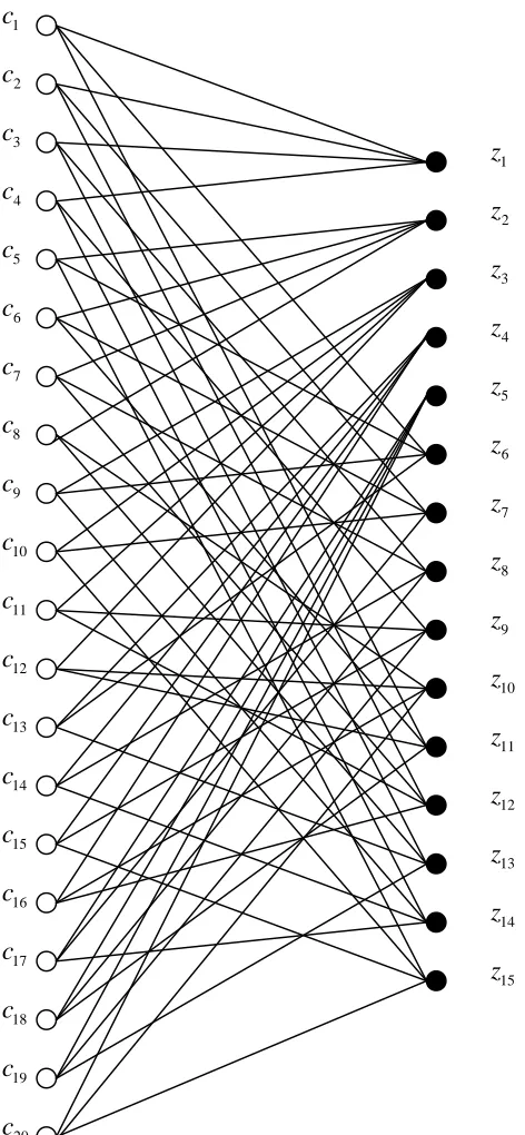
Figure 4.1 Tanner graph of Gallager’s (3, 4, 20) code. ... 66 Figure 4.2 Result of permutated rows and columns. ... 67 Figure 4.3 Performance of Gallager’s (3, 4, 20) code with iterative probabilistic

decoding. ... 74 Figure 5.1 Performance of parallel concatenated (turbo) code for different block

interleaver size with memory-4, rate-1/2 RSC codes and generators (37, 21). ... 78 Figure 5.2 Performance of rate-1/2 and rate- 1/3 parallel concatenated (turbo)

code with memory-2, generators (7, 5) block interleaver size = 1024 and iteration = 6. ... 79 Figure 5.3 Performance of rate-1/2 parallel concatenated (turbo) code with

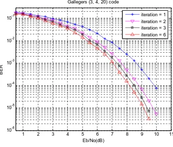
different constraint length. ... 81 Figure 5.4 Performance of Gallager’s (3, 4, 20) code with iterative probabilistic

decoding for different iteration number. ... 83 Figure 5.5 Performance of Gallager’s (3, 6, 96) code with iterative probabilistic

decoding for different iteration number. ... 84 Figure 5.6 Performance of Gallager’s (3, 6, 816) code with iterative

(11)

List of Tables

Page

Table 1 Quality of Service for rate 1/2 turbo code in AWGN at Eb/No = 3.0 dB. ... 80 Table 2 Quality of Service for rate 1/2 LDPC code in AWGN at Eb/No = 8.0 dB. ... 83 Table 3 Performance of a rate-1/2 parallel concatenated (turbo) code with

memory-4 rate-1/2 RSC codes, generators (37, 21). Block interleaver size = 102memory-4.

Iteration = 1. ... 164 Table 4 Performance of a rate-1/2 parallel concatenated (turbo) code with

memory-4 rate-1/2 RSC codes, generators (37, 21). Block interleaver size = 128.

(12)

Table 9 Performance of a rate-1/2 parallel concatenated (turbo) code with memory-4 rate-1/2 RSC codes, generators (37, 21). Block interleaver size = 256.

Iteration = 6. ... 166

Table 10 Performance of a rate-1/2 parallel concatenated (turbo) code with memory-4 rate-1/2 RSC codes, generators (37, 21). Block interleaver size = 2056. Iteration = 6. ... 166

Table 13 Performance of Gallager’s (3, 4, 20) code for iteration 1. ... 167

(13)

List of Appendices

Page

Appendix A ...91

Appendix B ...93

Appendix C ...96

(14)

Chapter 1

Introduction

In recent years, the demand for efficient and reliable digital data transmission and storage systems has increased to a great extent. The theory of error detecting and correcting codes is the branch of engineering and mathematics which deals with the reliable transmission and storage of data. Information media is not 100% reliable in practice, in the sense that noise frequently causes data to be distorted. To deal with this undesirable but inevitable situation, the concept of error control coding incorporates some form of redundancy into the digital data that allows a receiver to find and correct bit errors occurring in transmission and storage. Since such coding incurred in the communication or storage channel for error detection or error correction, it is often referred to as channel coding.

(15)

decoding can be defined as a technique employing a soft-output decoding algorithm that is iterated several times to provide powerful error correcting capabilities desired by very noisy wired and wireless channels. Turbo codes and low-density parity-check codes are two error control codes based on iterative decoding. The features of turbo codes include parallel code concatenation, recursive convolutional encoding, non-uniform interleaving, and an associated iterative decoding algorithm. Low-density parity-check (LDPC) codes are another method of transmitting messages over noisy transmission channels. LDPC code was the first code to allow data transmission rates close to the Shannon Limit, where Shannon limit of a communication channel is the theoretical maximum information transfer rate of the channel.

This chapter begins with a brief overview of wireless personal communications. The basic concepts of some error correcting codes other than iteratively decodable codes are then presented later in this chapter.

1.1

Wireless communications

An Italian electrical engineer, Guglielmo Marconi made the first wireless transmission across water in 1897. Wireless is an old-fashioned term for a radio transceiver. Radio transceiver is a mixed receiver and transmitter device. The original application of wireless was to communicate where wires could not go. Throughout the next century, great strides were made in wireless communication technology. During the First World War, the idea of broadcasting emerged, but broadcast stations were generally too awkward to be either mobile or portable. During the Second World War, the contest for superior battle field communication capabilities gave birth to mobile and portable radio.

(16)

waves are often unregulated. Wireless is now increasingly being used by unregulated computer users.

The development of mobile radio paved the way for personal communications. The first widespread non-military application of land mobile radio was pioneered in 1921 in Detroit, Michigan (Hamming 1950, pp. 147-160). The main purpose of it was to provide police car dispatch service. Until 1946, land mobile radio systems were unconnected to each other or to the Public Switched Telephone Network (PSTN). A major milestone was attained in 1946 with the development of the Radiotelephone in the U.S., which to be connected to the PSTN. At first, high powered transmitter and large tower were used to provide service to each market, and by this these markets could complete only one half-duplex call at a time. In 1950, Technological improvements doubled the number of concurrent calls, and the doubled the number again in the mid 1960’s. During that time, automatic channel trunking was introduced and full-duplex auto-dial service became available. However, the auto-trunked markets quickly became saturated. For example, in 1976, only 12 trunked channels were available for the entire New York City market of approximately 10 million people. The system could only support 543 paying customers and the waiting list exceeded 3700 people (Rappaport 1996).

1.1.1 Cellular communication systems

(17)

apart can be assigned the same frequency. The first operational commercial cellular system in the world was fielded in Tokyo in 1979 by NTT (Mitsishi 1989, pp. 30-39). Service in Europe soon followed with the Nordic Mobile Telephone (NMT), which was developed by Ericsson and began operation in Scandinavia in 1981(Kucar 1991, pp. 72-85). Service in the United States first began in Chicago in 1983 with the Advanced Mobile Phone System (AMPS), which was placed in service by Ameritech (Brodsky 1995).

By late 1980's, it was clear that the first generation cellular systems, which were based on analog signaling techniques, were becoming outdated. Progress in integrated circuit technology made digital communications not only practical, but more economical than analog technology. Digital communications allow the utilization of advanced source coding techniques that suit for greater spectral efficiency. Besides, with digital communications it is possible to use error correction coding to provide a degree of resistance to interference that plagues analog systems. Digital systems also enable multiplexing of dissimilar data types and more efficient network control.

Worldwide deployment of second generation digital cellular systems began in the early 1990's. The main difference to previous mobile telephone systems was that the radio signals that first generation networks used were analog, while second generation networks were digital. Second generation technologies can be divided into TDMA-based and CDMA-based standards depending on the type of multiplexing used. In the TDMA standard, also known as United States Digital Cellular (USDC)1, several users can transmit at the same frequency but at different times. In the CDMA standard, known initially as Interim Standard 95 (IS-95) and later as cdmaOne, several users can transmit at both the same frequency and time, but modulate their signals with high bandwidth spreading signals. Users can be separated in CDMA because the spreading signals are either orthogonal or have low crosscorrelation (Farely and Hoek M V D 2006).

Europe led the way in 1990 with the deployment of GSM (TDMA-based), the Pan European digital cellular standard. Before the deployment of GSM, there was no unified

(18)

standard in Europe. In Scandinavia there were two versions of NMT (NMT-450 and NMT-900), in Germany there was C-450, and elsewhere there was the Total Access Communication System (TACS) and R-2000 (Rappaport 1996), (Goodman 1997).

The situation in the United States was completely different than in Europe. In the U.S., there was but a single standard, AMPS. Since there was just one standard, there was no need to set aside new spectrum. However, the AMPS standard was becoming obsolete and it was obvious that a new technology would be required in crowded markets. The industry's response was to introduce several new incompatible, but bandwidth efficient, standards. Each of these standards was specified to be dual-mode systems. That is, they supported the original AMPS system along with one of the newer signaling techniques. Second generation systems in the U.S. can be divided into analog systems and digital systems. The second generation analog system is Narrowband AMPS (NAMPS), which is similar to AMPS except that the bandwidth required for each user is 10 kHz, rather than the 30 kHz required by AMPS (Farely and Hoek M V D 2006).

At the same time the 900 MHz band was being transitioned from AMPS to the new cellular standards. New spectrum became available in U.S. in the 1.9 GHz band. The systems that occupied this band used similar technology as their second generation siblings in the 900 MHz hand. Collectively, these systems were called Personal Com-munication Systems (PCS), implying a slightly different range of coverage and services than cellular (Farely and Hoek M V D 2006).

(19)

However, practical and economic factors limit just how much a cell can be emaciated. Each cell must be serviced by a centrally located base station. Base stations are expensive and require unsightly antenna towers. Many local governments block the placement of base station towers for reasons of aesthetics and perceived health risks. In addition, the network architecture is becoming more complex by increasing frequency due to occurrence of more cells.

1.1.2 Paging systems

While cellular telephony was evolving, progress was also made with other wireless devices and services including paging, wireless data, cordless telephony, and satellite telephony. Paging is considered as an important component of the growing wireless market. With paging, messages are sent in one way direction, from a centrally located broadcasting tower to a pocket sized receiver possessed by the end user.

Paging was the first mobile communication service for citywide paging systems and it was operating as early as 1963 in the USA and Europe. In the 1970's, with the emergence of the POCSAG (Post Office Code Standardization Advisory Group) standard, alphanumeric paging became possible. Initially POCSAG supported a simple beep-only pager but later incorporated numeric and alpha text messaging. Although the POCSAG standard was reliable, it operated at extremely low data rates so only short messages were permitted. New high speed standards have recently been installed and that allow faster transmission, and longer messages (Budde 2002).

(20)

1.1.3 Wireless data networks

Another emerging area of wireless communication technology is wireless data networks. The demand for wireless computer connectivity rises because of increasing popularity of both the Internet and laptop computers. Wireless data services are designed for packet-switched operation in contrast to the circuit-switched operation of cellular and cordless telephony. Each wireless data service can be categorized as either a wide-area messaging service or a wireless local area network (WLAN).

Wide-area messaging services use licensed bands, and customers pay operators based on their usage. Paging can be considered as a type of wide-area messaging service, although it is usually considered separately for historical reasons.Examples of messaging services include the Advanced Radio Data Information Service (ARDIS) and RAM Mobile Data (RMD). Both of them use the Specialized Mobile Radio (SMR) spectrum near 800/900 MHz (Padgett, Gunther and Hattori 1995, pp. 28-41).

(21)

1.1.4 Cordless telephony

“A cordless telephone or portable telephone is a telephone with a wireless handset which communicates with a base station connected to a fixed telephone landline (POTS) via radio waves and can only be operated close to (typically less than 100 meters of) its base station”.

(Cordless telephone 2006)

Cordless telephones were first emerged in the early 1980's as a consumer product. The benefit of cordless telephony is straight-forward, it allows the user to move around a house or business while talking on the phone, and it provides telecommunication service in rooms that might not be wired.

There are some limitations in first generation cordless phones. The analog signaling technique is prone to interference, spying, and fraud, especially as the number of users increased. In addition, the user is unable to use the phone when he or she goes out of the range of its base station. Modern cordless telephone standards have addressed these deficiencies. In the U.S.A, there are seven frequency bands that have been allocated by the Federal Communications Commission for uses and there are several proprietary cordless systems operating in the 900 MHz band. These systems use advanced digital signaling techniques such as spread spectrum. These are more robust against in-terference, and are more secure. In Europe, the DECT (Digital European Cordless Telephone) and CT-2 standards not only offer digital signaling, but allow connectivity beyond the home base station by employing a cellular-like infrastructure. A similar system in Japan, the Personal Handyphone System (PHS), has become extraordinarily successful (Rappaport 1996), (Goodman 1997).

(22)

1.1.5 Satellite telephony

Satellite telephony is similar to cellular telephony with the exception that the base stations are satellites in orbit around the earth. Depending on the architecture of a particular system, coverage may include the entire Earth, or only specific regions. Satellite telephony systems can be categorized according to the height of the orbit as either LEO (low earth orbit), MEO (medium earth orbit), or GEO (geosynchronous orbit).

GEO systems have been used for many years to communicate television signals. GEO telephony systems, such as INMARSAT, allow communications to and from remote locations, with the primary application being ship-to-shore communications. The advantage of GEO systems is that each satellite has a large footprint, and global coverage up to 75 degrees latitude can be provided with just 3 satellites (Padgett, Gunther and Hattori 1995, vol. 33, pp. 28-41). The disadvantage of GEO systems is that they have a long round-trip propagation delay of about 250 milliseconds and they require high transmission power (Miller 1998, vol. 35, pp. 26-35).

LEO satellites orbit the earth at high speed, low altitude orbits with an orbital time of 70– 90 minutes, an altitude of 640 to 1120 kilometres (400 to 700 miles), and provide coverage cells. With LEO systems, both the propagation time and the power requirements are greatly reduced, allowing for more cost effective satellites and mobile units (Satellite phone 2006).The main disadvantages of LEO systems are that more satellites are required and handoff frequently occurs as satellites enter and leave the field of view. A secondary disadvantage of LEO systems is the shorter lifespan of 5-8 years (compared to 12-15 in GEO systems) because of increasing amount of radiation in low earth orbit (Miller 1998, vol. 35, pp. 26-35).

(23)

startup), as well as the proposed Teledesic system (288 satellites, 2002 startup). Examples of MEO systems include ICO (10 satellites, 2000 start up), and TRW's Odyssey (12 satellites, 1998 startup) (Miller 1998, vol. 35, pp. 26-35).

1.1.6 Third generation systems

3G is short for third-generation technology. It is used in the context of mobile phone standards. At the close of the 20th century, mobile communications are characterized by a diverse set of applications using many incompatible standards.

In order for today's mobile communications to become truly personal communications in the next century, it will be necessary to consolidate the standards and applications into a unifying framework. The eventual goal is to define a global third generation mobile radio standard originally termed the Future Public Land Mobile Telecommunications System (FPLNITS), and later renamed for brevity IMT-2000, for International Mobile Telecommunications by the year 2000 (Berruto, Gudmundson, Menolascino, Mohr and Pizarosso 1998, vol. 36, February, pp. 85-95).

1.2

Other applications of error control coding

(24)

1.2.1 Hamming codes

Hamming codes are the first class of linear codes devised for error correction (Hamming 1950, pp. 147-160). These codes and their variations have been widely used for error control in digital communication and data storage system. The fundamental principal embraced by Hamming codes is parity. Hamming codes are capable of correcting one error or detecting two errors but not capable of doing both simultaneously.

For any positive integer m≥3, there exists a Hamming code with the following parameters.

Code length: n=2m −1

Number of information symbols: 2m 1

k= − −m

Number of parity-check symbols: n k− =m

Error-correcting capability: t=1, where, d_min =3.

A Hamming code word is generated by multiplying the data bits by generator matrix G using modulo-2 arithmetic. This multiplication's result is called the code word vector

1 2

( ,c c ,K,c_n)consisting of the original data bits and the calculated parity bits.

The generator matrix G is used in constructing Hamming codes consists of I (the identity matrix) and a parity generation matrix A:

[ : ]

G= I A (1.1)

(25)

1.2.2 The binary Golay code

The binary form of the Golay code is one of the most important types of linear binary block codes. It is of particular significance, since it is one of only a few examples of a nontrivial perfect code. A t-error-correcting code can correct a maximum number of t errors. One of the major properties of a perfect t-error-correcting code is that every word lies within a distance of t to exactly one code word.

Equivalently, the code has minimum distance, dmin = +2t 1, and covering radius t, where the

covering radius r is the smallest number such that every word lies within a distance of r to a codeword.

There are two closely related binary Golay codes. The extended binary Golay code encodes 12 bits of data in a 24-bit word in such a way that any triple-bit error can be corrected and any quadruple-bit error can be detected. The second one, the perfect binary Golay code, has codewords of length 23 and is obtained from the extended binary Golay code by deleting one coordinate position. Conversely, the extended binary Golay code can be obtained from the perfect binary Golay code by adding a parity bit (Morelos-Zaragoza 2002).

1.2.3 Binary cyclic codes

Cyclic codes form an important subclass of linear codes. These codes are attractive for two reasons: first, they can be efficiently encoded and decoded using simply shift-registers and combinatorial logic elements, based on their representation using polynomials; and second, because they have considerable inherent algebraic structure.

(26)

BCH codes are family of cyclic codes. A BCH (Bose, Ray-Chaudhuri, Hocquenghem) code is a much studied code within the study of coding theory and more specifically error-correcting codes. In technical terms, a BCH code is a multilevel, cyclic, error-error-correcting, variable-length digital code that is used to correct multiple random error patterns.

1.3

Purpose and structure of thesis

It is well known that wireless links are very vulnerable to channel imperfection such as channel noise, multi-path effect and fading. Iterative decoding is a powerful technique to correct channel transmission errors, and thus improve the bandwidth efficiency of wireless channels.

The essential idea of iterative decoding is to use two or more soft-in/soft-out (SISO) component decoders to exchange soft decoding information. This soft decoding information is known as extrinsic information. It is the exchange of the extrinsic information that provides the powerful error correcting capabilities desired by very noisy wired and wireless channels.

Turbo codes and low-density parity-check (LDPC) codes are two error control codes based on iterative decoding. These codes are widely used in various international standards, such as W-CDMA, CDMA-2000, IEEE 802.11, and DVB-RCS. The purpose of this study is to investigate the performance of two error control codes, namely, turbo codes and LDPC codes based on iterative decoding and demonstrate the performance comparison between these two codes, in terms of error resilient performance, latency, and computational resources. In the first part of this thesis, the fundamental of wireless networks were presented along with some brief explanation of other error control codes. Chapter 2 begins with the history of turbo codes and LDPC codes, and then gives an overview of block, convolutional and concatenated codes.

(27)

(28)

Chapter 2

Error correction coding

(29)

construction and the algorithms that are used to decode turbo codes and LDPC codes are detailed in the following chapters.

2.1

History

Iterative decoding technique was first introduced in 1954 by P. Elias when he showed his work on iterated codes in his paper “Error-Free Coding” (Elias 1954, vol. PGIT-4, pp. 29-37). Later, in the 1960s, R. G. Gallager and J. L. Massey made an important contribution. In their papers, they referred to iterative decoding as probabilistic decoding (Gallager 1962, vol. 8, no. 1, pp. 21-28), (Massey 1963). The main concept then and as it is today, is to maximize the a-posteriori probability of sending data which is a noisy version of the coded sequence.

Over the past eight years, a substantial amount of research effort has been committed to the analysis of iterative decoding algorithms and the construction of iteratively decodable codes or “turbo-like codes” that approach the Shannon limit. Turbo codes were introduced by C. Berrou, A. Glavieux and P. Thitimajshima in their paper “Near Shannon

Limit Error-Correcting Coding and Decoding: Turbo- Codes” in 1993 (Berrou, Glavieux

& Thitimajshima 1993, pp. 1064-1070).

(30)

algorithm with almost linear complexity (Zyablov & Pinsker 1975, vol. 11, no. 1, pp. 26-36). D. J. C. MacKay and R. M. Neal have showed that LPDC codes can get close to the Shannon limit as turbo codes (MacKay & Neal 1996, vol. 32, pp. 1645-1646). Later in 2001, T. J. Richardson, M. A. Shokrollahi and R. L. Urbanke have showed irregular LPDC codes may outperform turbo codes of approximately the same length and rate, when the block length is large (Richardson, ShokroLLahi & Urbanke 2001, vol. 47, no. 2, pp. 619-637).

However, such codes have been studied in detail only for the most basic communication system, in which a single transmitter sends data to a single receiver over a channel whose statistics are known to both the transmitter and the receiver. Such a simplistic model is not valid in the case of wireless networks, where multiple transmitters might want to communicate with multiple receivers at the same time over a channel which can vary rapidly. While the design of efficient error correction codes for a general wireless network is an extremely hard problem and hence the techniques of iterative decoding are still under experimentation and study.

2.2

Basic concepts of error correcting coding

(31)

errors at an acceptably low level. Figure 2.1 shows the representation of a typical transmission by a block diagram.

All error correcting codes are based on the same basic principles. The encoder takes the information symbols from the source as input and adds redundant symbols to it. In a basic form, redundant symbols are appended to information symbols to obtain a coded sequence or codeword. Most of the errors that are introduced during the process of modulating a signal, transmission over a noisy medium and demodulation, can be corrected with the help of those redundant symbols. Such an encoding is said to be systematic. Figure 2.2 shows the systematic block encoding for error correction, where first k symbols are information symbols and remaining n-k symbols are some functions of the information symbols. These

n-k redundant symbols are used for error correction or detection purposes. The set of all code

[image:31.595.110.526.412.618.2]

sequence is called an Error Correcting Code (ECC) and it is denoted by C.

Figure 2.1: A digital communication system.

Encoder Modulation

ECC

Noisy Medium

Information destination

CODED

MODULATION

u

Information source

v

x

y

r

u

%

(32)

Figure 2.2: Systematic block encoding for error correction.

2.3

Shannon capacity limit

In 1948, Claude E. Shannon published his era making paper (Shannon 1948, vol. 27, pp. 379-423 and 623-656) on the limits of reliable transmission of data over unreliable channels and methodologies of achieving these limits. In that paper, he also formalized the concept of information and investigated bounds for the maximum amount of information that can be transmitted over unreliable channels. In the same paper Shannon introduced the concept of codes as ensembles of vectors that are to be transmitted.

Form Figure 2.1, let’s assume the information source produces a message { }, _i _i {0,1}, 0 1

u = u u ∈ ≤ ≤ −i k , of k data bits. The data bits are passed through a channel encoder, which adds structured redundancy by performing a one-to-one mapping of the message u to a code word x ={ }, x_i x_i∈{X₀,X₁}, 0≤ ≤ −i n 1 of n code symbols, where

0

X and X are symbols suitable for transmission over the channel. Hence, the code has a ₁

rate of r = k/n bits per symbol. The codeword x is transmitted over a channel with some capacity bits per channel use.

Given a communication channel, Shannon proved that there exists a number, called the capacity of the channel, such that reliable transmission is possible for rates arbitrarily close to the capacity, and reliable transmission is not possible for rates above the capacity.

n - k symbols k symbols

n symbols

(33)

The channel capacity depends on the type of channel and it measures the number of data bits that can be supported per channel use (Shokrollahi 2003, pp.2-3).

Now, let’s presume the received version of the codeword y is passed through a channel

decoder, which estimates u% of the message. If the channel allows for errors, then there is no general way of telling which codeword was sent with absolute certainty. However, one way to find the most likely codeword is simply list all the 2k

possible codewords, and calculate the conditional probability for the individual codewords. Then find the vector or vectors that yield the maximum probability and return one of them. This decoder is called the maximum likelihood decoder.

Shannon proved a random code can achieve channel capacity for sufficient long block lengths. However, random codes of sufficient length are not practical to implement. Practical codes must have some structure to allow the encoding and decoding algorithms to be executed with reasonable complexity. Codes that approach capacity are very good from a communication point of view, but Shannon's theorems are non-constructive and don't give a clue on how to find such codes (Shokrollahi 2003, pp.2-3).

2.4

Block codes

(34)

then calculate three check bits which are a linearly combination of the information bits. The resulting seven bits code word was then fed into the computer. After reading the resulting codeword, the computer ran through an algorithm that could not only detect errors, but also determine the location of a single error. Thus the Hamming code was able to correct a single error in a block of seven encoded bits (Hamming 1950, pp. 147-160).

Although Hamming codes were a great progression, it had some undesirable proper-ties. Firstly, it was not very efficient. It was requiring three check bits for every four data bits. Secondly, it had the ability to correct only a single error within the block. These problems were addressed by Marcel Golay, who generalized Hamming's construction. During his process, Golay discovered two very astonishing codes on which the binary Golay code has already mentioned concisely in Section 1.2.2. The second code is the ternary Golay code, which operates on ternary, rather than binary, numbers. The ternary Golay code protects blocks of six ternary symbols with five ternary check symbols and has the capability to correct two errors in the resulting eleven symbol code word (Golay 1949, vol. 37, p. 657).

The general strategy of Hamming and Golay codes were the same. The ideas were to group q-ary symbols into blocks of k-digit information word and then add n-k redundant symbols to produce an n-digit code word. The resulting code has the ability to correct t errors, and has code rate r = k/n. A code of this type is known as a block code, and is referred to as a (q, n, k, t) block code.

2.5

Convolution codes

(35)

frame synchronization.2 Thirdly, most of the algebraic-based decoders for block codes work with bit decisions, rather than with "soft" outputs of the demodulator. With hard-decision decoding, the output of the channel is taken to be binary, whereas the channel output is continuous-valued with soft-decision decoding. However, in order to achieve the performance bounds predicted by Shannon, continuous-valued channel output are required.

The drawbacks of block codes can be avoided by taking a different approach to coding and one of them was convolutional coding. Convolutional codes were first introduced in 1955 by Elias (Elias 1955, vol. 4, pp. 37-47). Rather than splitting data into distinct blocks, convolutional encoders add redundancy to a continuous stream of input data by using a linear shift register. In convolutional codes, each block of k bits is mapped into a block of n bits but these n bits are not only determined by the present k information bits but also by the previous information bits. This dependence can be captured by a finite state machine. The total number of bits that each output depends on is called the constraint length, and denoted by Kc. The rate of the convolutional encoder is the number of data bits k taken in by the

encoder in one coding interval, divided by the number of n coded bits during the same interval. While the data is continuously encoded, it can be continuously decoded with only small latency. In addition, the decoding algorithms can make full rise of soft-decision information from the demodulator.

After the development of the Viterbi algorithm, convolutional coding began to be utilized in extensive application of communication systems. The constraint length Kc = 7

"Odenwalder" convolutional code, which operates at rates r = 1/3 and r = 1/2, has become a standard for commercial satellite communication applications (Berlekamp, Peile and Pope 1987), (Odenwalder 1976). Convolutional codes were used by several deep space probes such as Voyager and Pioneer (Wicker 1995).

All of the second generation digital cellular standards incorporate convolutional coding; GSM uses a Kc = 5, r = 1/2 convolutional code, USDC use a Kc = 6, r = 1/2 convolutional

code, and IS-95 uses a Kc = 9 convolutional code with r = 1/2 on the downlink and r = 1/3

2_{Frame synchronization means that the decoder has knowledge of which symbol is the first symbol in a}

(36)

on the uplink (Rappaport 1996). Globalstar also uses a Kc = 9, r = 1/2 convolutional code,

while Iridium uses a Kc = 7 convolutional code with r = 3/4 (Costello, Hagenauer, Imai and

Wicker 1998, vol. 44, pp. 2531-2560).

2.6

Concatenated codes

Convolutional codes have a key weakness and that is vulnerability to burst errors. This weakness can be eased by using an interleaver, which scrambles the order of the coded bits prior to transmission. At the receiver end, a deinterleaver is used that places the received coded bits back into the proper order after demodulation and prior to decoding. The most common type of interleaver is the block interleaver, which is simply an Mb x Nb bit array.

Data is placed into the array column-wise and then read out row-wise. A burst error of length up to Nb bits can be spread out by a block interleaver such that only one error occurs

in every Mb bits. All of the second generation digital cellular standards use some form of

block interleaving. A second type of interleaver is the convolutional interleaver, which allows continuous interleaving and deinterleaving and is ideally suited for use with convolutional codes (Ramesy 1970, vol. 16, pp. 338-345).

2.7

Iterative decoding for soft decision codes

(37)

2.7.1 Turbo codes

Turbo codes are a new class of error correction codes that was introduced in 1993, by a group of researchers from France, along with a practical decoding algorithm. The turbo codes are very important in the sense that they enable reliable communications with power efficiencies close to the theoretical limit predicted by Claude Shannon. Hence, turbo codes have been projected for low-power applications such as deep-space and satellite communications, as well as for interference limited applications such as third generation cellular and personal communication services. Figure 2.3 shows the block diagram of turbo encoder.

Figure 2.3: Encoder structure of a parallel concatenated (turbo) code.

A turbo code is the parallel concatenation of two or more Recursive Systematic Convolutional (RSC) codes separated by an interleaver. Two identical rate r = 1/2 RSC encoders work on the input data in parallel as shown in Figure 2.3. As shown in the figure, the upper encoder receives the data directly, while lower encoder receives the data after it has been interleaved by a permutation function α. In general, the interleaver α is a pseudo-random interleaver. It maps bits in position i to position

( )i

α according to a prescribed, but randomly generated rule. Because the encoders

Parity Output Systematic Output

Data Upper RSC

Encoder

Lower RSC Encoder Interleaver

(38)

are systematic (one of the outputs is the input itself) and receive the same input (although in a different order), the systematic output of the lower encoder is completely unnecessary and does not need to be transmitted. However, the parity outputs of both encoders are transmitted. The overall code rate of the parallel concatenated code is r = 1/3, although higher code rate can be achieved by

puncturing the parity output bit with a multiplexer (MUX) circuit.

Figure 2.4: Block diagram of an iterative decoder for a parallel concatenated code.

As an interleaver exists between two encoders, optimal decoding of turbo codes is incredibly complex and therefore impractical. However, a suboptimal iterative decoding algorithm was presented in (Berrou, Glavieux & Thitimajshima 1993, pp. 1064-1070) which presents good performance at much lower complexity. The idea behind the decoding strategy is to break the overall decoding problem into two smaller problems with locally optimal solutions and to share information in an iterative fashion. The decoder associated with each of the constituent codes is modified so that it produces soft-outputs in the form of a-posteriori probabilities of

Systematic Data

Parity Data

Decoded output

Upper Decoder

Lower Decoder Interleaver

DeMUX

Deinterleaver

(39)

the data bits. The two decoders are cascaded as shown in Figure 2.4. As shown in the figure, the lower decoder receives the interleaved version of soft-output of the upper decoder. At the end of the first iteration, the deinterleaved version of soft-output of the lower decoder is fed back to the upper decoder and used as a-priori information in the next iteration. Decoding continues in an iterative fashion until the desired performance is achieved.

The original turbo code of (Berrou, Glavieux & Thitimajshima 1993, pp. 1064-1070) used constraint length Kc = 5 RSC encoders and a 65,536 bit interleaver. The parity

bits were punctured in such a way that the overall code was a (n = 131,072, k =

65,532) linear block code. Simulation results showed that a bit error rate of 5

10− could be achieved at an E_b/N ratio of just 0.7 decibels (dB) after 18 iterations of ₀

decoding. Thus, the author claimed that turbo codes could come within a 0.7 dB of the Shannon limit. However, it is found that the performance of the turbo codes increases as the length of the codes n increases.

2.7.2 LDPC codes

LDPC codes are one of the hottest topics in coding theory today. Besides turbo codes, low-density parity-check (LDPC) codes form another class of Shannon limit-approaching codes. Unlike many other classes of codes, LDPC codes are very well equipped with very fast encoding and decoding algorithms by now. The design of the codes is such that these algorithms can recover the original codeword in the face of large amount of noise. New analytic and combinatorial tools make LDPC codes not only attractive from a theoretical point of view, but also perfect for practical applications.

(40)

they have been strongly promoted, and MacKay in his work showed that LDPC codes are capable of closely approaching the channel capacity. In particular, using random coding arguments MacKay showed that LDPC code collections can approach the Shannon capacity limit exponentially fast with increasing code length (MacKay & Neal 1996, vol. 32, pp. 1645-1646).

LDPC codes are codes, specified by a matrix containing mostly 0’s and relatively few 1’s. There are basically two classes of LDPC codes based on the structure of this matrix, i.e., regular LDPC codes and irregular LDPC codes.

A regular LDPC code is a linear (w w N code with parity-check matrix H having the c, r, ) Hamming weight of the columns and rows of H is equal to w and _c w , where both _r w and _c

r

w are much smaller than the code length N. In somewhat artificial sense, LDPC codes are

not most favorable of minimizing the probability of decoding error for a given block length. It can be shown that the maximum rate at which they can be used is bounded by the channel capacity. However, the simplicity in the decoding scheme can compensate these disadvantages.

As previously mentioned, a regular LDPC code is defined as the null space of a parity-check matrix H. This parity-check matrix has some structural properties which are given

below:

1. The parity-check matrix H has constant Hamming weight of the columns and rows equal to w and _c w , where both _r w and _c w are much smaller than the code _r

length.

2. The number of 1’s in common between any two columns, denoted by λ, is no greater than 1. This implies that no two rows of H have more than one 1 in common. Because both w and _c w are small compared with the code length and _r

(41)

This is the reason why H is said to be a low-density parity-check matrix, and the code specified by H is hence called a low-density parity check (LDPC) code.

An irregular LDPC codes are obtained, if the Hamming weights of the columns and rows of H are chosen in accordance to some nonuniform distribution (Richardson, ShokroLLahi & Urbanke 2001, vol. 47, no. 2, pp. 619-637). An irregular LDPC code has a very sparse parity check matrix in which the column weight may vary from column to column. In fact, the best known LDPC codes are irregular; they can do better than regular LDPC codes by 0.5 dB or more (Luby, M G, Miteznmacher, Shokrollahi, M A and Spielman, D A 2001, vol. 47, no. 2, pp. 585-598).

2.8

Chapter summary

This chapter has focused on the basic concepts of two classes of ECC codes, i.e., turbo codes and LDPC codes. Both turbo codes and LDPC codes utilize a soft-output decoding algorithm that is iterated several times to improve the bit error probability, with the aim of approaching Shannon capacity limit, with less complexity.. The basic concepts of error correcting codes and Shannon capacity limit were presented. Turbo codes have many of the common concepts and terminologies of block codes, convolutional codes and concatenated codes. LDPC codes also share some idea of block codes. Hence, an outline for each block codes, convolutional codes and concatenated codes was presented separately.

(42)

Chapter 3

Turbo codes: Encoder and decoder construction

This chapter focuses on the encoder construction and decoding algorithms of turbo codes. Turbo codes share many of the same concepts and terminologies of both block codes and convolutional codes. For this reason, it is helpful to first provide an overview of block codes and convolutional codes before proceeding to the discussion of turbo coeds.

3.1

Constituent block codes

Block codes process the information on a block-by-block basis, treating each block of information bits independently from others. Typically, a block code takes a k-digit

information word, and transforms this into an n-digit codeword. At first, the encoder for a

block code divides the information sequence into message blocks of k information bits

each. A message block is then represented by the binary k-tuple u = (u0, u1, …, uk-1). So

(43)

independently into an n-tuple v = (v0, v1,…,vn-1 ). Hence, corresponding to the 2k

different possible messages, there are 2n different possible code words at the encoder

output.

3.1.1 Encoding of block codes

The encoding process consists of breaking up the data into k-tuples u called messages,

and then performing a one-to-one mapping of each message ui to an n-tuple vi called a

code word. Let C denote a binary linear (n, k, dmin) code. Since C is a k-dimensional

vector subspace, any codeword v∈Ccan be represented as a linear combination of the elements in the basis:

0 0 1 1 k 1 k 1,

v =u v +u v + +L u ₋v ₋ (3.1)

where u_i∈{0,1}, 0≤ < −i k 1. Equation (3.1) can be described by the matrix multiplication

,

v =uG (3.2)

where G is the k × n generator matrix.

0,0 0,1 0, 1

0

1,0 1,1 1, 1

1

1,0 1,1 1, 1

1

.

n n

k k k n

k

v v v

v

v v v

v G

v v v

v

−

− − − −

−

 

 

=_ _=_ _

 

 _{ } _

   

L L

M M M

M O

L

(3.3)

Since C is k-dimensional vector space in V2, there is an (n - k) - dimensional dual

(44)

The Hamming distance dH( ,v v1 2) is the number of positions that two code words differ.

It can be found by first taking the modulo-2 sum of the two code words and then counting the number of ones in the result. The minimum distance dmin of a code is the smallest Hamming distance between any two words

1 2

min _{v v}min {_, _C H( ,1 2) | 1 2}.

d d v v v v

∈

= ≠ (3.4)

A code with the minimum distance dmin is capable of correcting all code words with t or fewer errors, where

min 1 _,

2

d t=_ − _

  (3.5)

where x   denotes the largest integer less than or equal to x.

The Hamming weight can be found by simply counting the number of ones in the code word. For linear codes, the minimum distance is the smallest Hamming weight of all code words except the all-zeros code word

min 0

( ).

min

i

d w v

>

= (3.6)

3.1.2 Systematic codes

A code is said to be systematic if the message u is contained within the codeword v . The generator matrix G of a systematic code can be brought to systematic form

[ | ],

sys k

(45)

where I is the k × k identity matrix and P is a k × (n - k) parity sub-matrix, such that k

0,0 0,1 0, 1

1,0 1,1 1, 1

.

n k n k

k k k n k

p p p

P

p p p

− −

− − − − −

 

 

=_ _

 

 

L L

M M O M

L

(3.8)

Since GHΤ =0, it follows that the systematic form, H_sys, of parity-check matrix is

[ | |].

sys n k

H = PΤ I ₋ (3.9)

3.2

Constituent convolution codes

3.2.1 Encoding of convolution codes

A convolution encoder has memory, in the sense that the output symbols depend not only on the input symbols, but also on the previous inputs or outputs. The memory m of the encoder measured by the total length of shift registers M. Constraint length Kc = m + 1, is

defined as the number of inputs (u[i], u[i-1], … u[i-m]) that affect the outputs (

v(0)[i],…,v(n-1)[i]) at time i. An encoder with m memory elements will be referred to as a

(46)

Figure 3.1: An encoder of memory-2 rate-1/2 convolutional encoder.

3.2.2 State diagram

A memory-m rate 1/n convolution encoder can be represented by a state diagram. An encoder with m memory elements there are 2m states. Figure 3.2 shows the state diagram of the memory-2 rate- 1/2 convolution code. As there is only one information bit, hence two branches enter and leave each state and they are labeled by u[i] / v(0)[i],…,v(n-1)[i].

Figure 3.2: State diagram of a memory-2 rate-1/2 convolutional encoder. v (1)

v (0)

+ +

+

S0 S1

u

0/01

1/01 0/10

1/00 0/11

1/11 0/00

00

11 10

01

(47)

3.2.3 Generator matrix

For an encoder with memory -m rate-1/2, the impulse responses can last at most m + 1 time units and can be written as (0) (0) (0) (0)

0 1

( , , , _m )

g = g g L g and (1) (1) (1) (1)

0 1

( , , , _m )

g = g g L g . The impulse responses g(0) and g(1) are called the generator sequences of the encoder. In general, when referring to a convolution code, the generators are expressed in octal form. In order to stress the dynamic nature of the encoder, the indeterminate D (for “Delay”) is used and the generators are written as polynomials in D, g(0)( ),D L,g(n−1)( )D .

A convolutional encoder is a linear time-invariant system, with impulse responses given by the code generators, (0) ( 1)

( ), , n ( )

g D L g − D , where

( ) ( ) ( ) ( ) 2 ( )

0 1 2

( ) ,

j j j j j m

m

g D =g +g D+g D + +L g D (3.10)

for 0≤ <j n. In term of the generators of a code, the output sequences can be expressed as ( )

[ ]

0 [ ] [ ] m j j l

v i u i l g l

=

∑

− , where 0≤ <j n (3.11)

In particular, for a rate-1/2 memory-m encoder, if the generator sequences (0) g and

(1)

g are interlaced, then they can be arranged in the matrix in such that

(0) (1) (0) (1) (0) (1) (0) (1)

0 0 1 1 2 2

(0) (1) (0) (1) (0) (1) (0) (1)

0 0 1 1 1 1

(0) (1) (0) (1) (0) (1) (0) (1)

0 0 2 2 1 1

... ... ... ... ... ... ... m m

m m m m

m m m m m m

g g g g g g g g

G g g g g g g g g

(48)

where the blank areas are all zeros. We can then, write the encoding equations in matrix form as

v =uG, (3.13)

where all operations are modulo-2. The G matrix is then called the Generator matrix of the encoder.

Hence, the output sequences v( )j ( ), 0D ≤ <j n, as mentioned, are equal to the discrete convolution between the input sequence u D and the code generators ( )

(0) (1) ( 1)

( ), ( ), , n ( )

g D g D L g − D . Let, v D( )=v(0)( )D +Dv(1)( )D + +L Dn−1 (vn−1)( )D . Then the relationship between input and output can be written as follows:

( ) ( ) ( ),

v D =u D G D (3.14)

where, generators of a rate 1/n convolutional code are arranged in matrix and referred to as a polynomial generator matrix ( )G D .

3.2.4 Trellis diagram

(49)

[image:49.595.127.523.116.337.2]

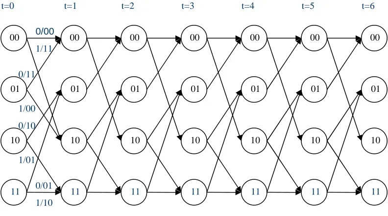
Figure 3.3: Six sections of the trellis of a memory-2 rate-1/2 convolutional encoder.

3.2.5 Punctured convolution codes

If convolutional codes are rate of 1/n, the highest rate that can be achieved is r = 1/2. For many applications it may be desirable to have higher rates such as r = 2/3 or r = 3/4. One way to attain these higher rates is to use an encoder that can take more than one input stream and thus having rate r = k/n, where k > 1. However, this increases the complexity of decoder’s add-compare-select (ACS) circuit exponentially in the number of input streams (Wicker 1995). Hence, it is desirable to keep the number of input streams at the encoder as low as possible. An alternative of using multiple encoder input streams is to use a single encoder input stream and a process called puncturing.

Puncturing is the process of systematically deleting, or not sending some output bits of a low-rate encoder. The code rate is determined by the number of deleted bits. For instance, one out of every four bits is deleted from the output of a rate 1/2 convolutional encoder. Then for every two bits at the input of the encoder, three bits remain as outputs after puncturing. Hence, the punctured rate is 2/3. The convolutional codes of rate 3/4 can be

1/10 0/01 1/01 0/10 1/00 0/11

1/11

0/00

t=0 t=1 t=2 t=3 t=4

00

01

10

11

00 00 00 00 00 00

01 01 01 01 01 01

10 10 10 10 10 10

11 11 11 11 11 11

(50)

generated from the same encoder by deleting two out of every six output bits. One of the main benefits of puncturing is that it allows the same encoder to attain a wide range of coding rates by simply changing the number deleted bits (Hagenauer 1988, vol. 36, pp. 389-400).

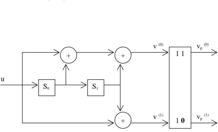
When puncturing is used, the location of the deleted bits must be explicitly stated. A puncturing matrix P specifies the rules of deletion of output bits. P is a k × np binary matrix,

with binary symbols pij that indicate whether the corresponding output bit is transmitted (pij

= 1) or not (pij = 0). For example, the following matrix can be used to increase a rate 1/2

code to rate 2/3

1 1 1 0

P=_ _

[image:50.595.127.478.361.574.2]

 

Figure 3.4: An encoder of a memory-2 rate-2/3 PCC.

The corresponding encoder is depicted in Figure 3.4. A coded sequence

(0) (1) (0) (1) (0) (1) (0) (1)

1 1 2 2 3 3

(..., i i , i i , i i , i i ,...)

v = v v v v₊ ₊ v v₊ ₊ v v₊ ₊ _,

vp(1)

vp(0)

v (1)

v (0)

+ +

+

S0 S1

1 1

1 0

(51)

of the rate- 1/2 encoder is transformed into code sequence

(0) (1) (0) (0) (1) (0)

1 2 2 3

(..., , , , ,...)

p i i i i i i

v = v v v₊ v v₊ ₊ v₊ ,

i.e., every other bit of the second output is deleted (Morelos-Zaragoza 2002).

One of the goals of puncturing is that for a variety of high-rate codes, the same decoder can be used. One way to achieve decoding of a punctured convolution code using the viterbi decoder of the low-rate code is by the insertion of “deleted” symbols in the positions that were sent. This process is known as depuncturing. A special flag is used to mark these deleted symbols.

3.2.6 Recursive systematic codes

[image:51.595.119.494.469.674.2]

If a data sequence being encoded becomes a part of the encoded output sequence, that codes are referred to as systematic.

Figure 3.5: An encoder of a memory-2 rate-1/2 recursive systematic convolutional encoder.

(1)

i

v (0)

i

v

i

u

S

S0 S1

+

(52)

Convolutional codes can be made systematic without reducing the free distance. A rate 1/2 convolutional code is made systematic by first calculating the remainder ( )y D of the

polynomial division u D( ) /g(0)( )D . The parity output is then found by the polynomial

multiplication v(1)( )D =y D g( ) (1)( )D , and the systematic output is simply

(0)

( ) ( )

v D =u D . Codes generated in this manner are referred to as recursive systematic convolutional (RSC) codes. RSC encoding proceeds by first computing the remainder variable

0 1

[ ] [ ] [ ] [ ]

m l

y i u i y i l g l

=

= +

∑

− (3.15)

and then finding the parity output

(1)

1 0

[ ] [ ] [ ]

m l

v i y i l g l

=

∑

− (3.16)

(53)

[image:53.595.131.524.403.626.2]

Figure 3.6: State diagram of a memory-2 rate-1/2 recursive systematic convolutional encoder.

Figure 3.7: Six sections of the trellis of a memory-2 rate-1/2 recursive systematic convolutional encoder.

0/01

0/01 1/10

0/00 1/11

1/11 0/00

00

11 10

01

1/10

1/10 0/01 0/01 1/10 0/00 1/11

1/11 0/00

t=0 t=1 t=2 t=3 t=4

00

01

10

11

00 00 00 00 00 00

01 01 01 01 01 01

10 10 10 10 10 10

11 11 11 11 11 11

(54)

It can be noticed that the state and the trellis diagrams for the RSC code are almost identical to those for the related non-systematic convolutional code. Actually, the only difference between the two state diagrams is that the input bits labeling the branches leaving nodes (10) and (01) are complements of one another. In conventional convolutional codes, the input bits labeling the two branches entering any node are the same. Conversely, for RSC codes, the input bits labeling the two branches entering any node are complements of one another. Since the structure of the trellis and the output bits labeling the branches remain the same when the code is made systematic and the minimum free distance remain unchanged.

3.3

Classes of soft-input, soft- output decoding algorithms

3.3.1 Viterbi algorithm

Viterbi Algorithm (VA) is the optimu