An adaptive data filtering model for remaining useful life estimation

(1)

warwick.ac.uk/lib-publications

A Thesis Submitted for the Degree of PhD at the University of Warwick

Permanent WRAP URL:

http://wrap.warwick.ac.uk/106052

Copyright and reuse:

This thesis is made available online and is protected by original copyright. Please scroll down to view the document itself.

Please refer to the repository record for this item for information to help you to cite it. Our policy information is available from the repository home page.

(2)

M A

E

G NS

I T A T MOLEM

U N

IV

ER

SITAS WARWIC EN

SIS

An Adaptive Data Filtering Model for

Remaining Useful Life Estimation

by

Oguz BEKTAS

Thesis

Submitted to the University of Warwick

for the degree of

Doctor of Philosophy

Warwick Manufacturing Group

(3)

List of Tables

2.1 Classification of Maintenance . . . 12

2.2 Physics Based Models . . . 33

2.3 Knowledge Based Models . . . 37

2.4 Data-driven Prognostics . . . 41

2.5 ANN-based Prognostics in Complex Systems . . . 55

2.6 Comparison of Prognostic Approaches . . . 70

4.1 PHM08 challenge data set parameters available to participants as sensor data . . . 130

4.2 Number of trajectories and regimes in C-MAPSS data sets . . 131

4.3 Corresponding values for regimes . . . 138

4.4 Results of Prognostic Parameter Suitability Metrics . . . 141

4.5 Distribution of PHM08 Final Test Trajectories According to Operational Length . . . 153

5.1 Prognostic Metrics . . . 174

5.2 RUL estimation range for the units with lowest performance . 177 5.3 Secondary Dataset#1 RUL estimations with lowest performance 178 5.4 Prognostic metrics for Secondary Data set #1 with different window sizes used for HI moving average filtering . . . 182

(8)

5.6 Secondary Dataset#12 RUL estimations with lowest performance183

5.7 Performance Evaluation of Secondary Datasets . . . 186

5.8 Prognostic Performance of the Presented Model . . . 188

5.9 Previous Leader board of the “final data set” of PHM08 . . . 188

A.1 Performance of selected approaches . . . 237

A.2 PHM08 Data Challenge Leader board . . . 238

(9)

List of Figures

2.1 Major Steps in CBM . . . 17

2.2 Failure progression timeline . . . 26

2.3 System life model . . . 27

2.4 A Typical Prognostic Application . . . 29

2.5 Prognostic Terms . . . 30

2.6 A single neuron . . . 59

2.7 A single neurone with multiple inputs . . . 60

2.8 A multiple-layer neural network . . . 61

2.9 Characteristic of Scoring Function . . . 81

3.1 Multidimensional Data . . . 92

3.2 Stages of the Methodology . . . 100

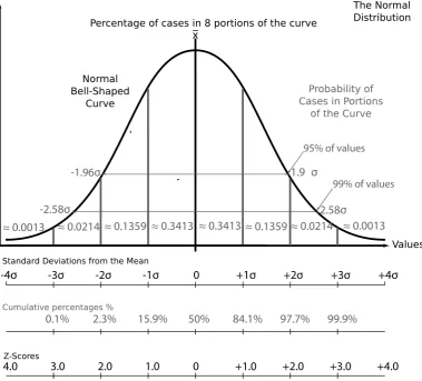
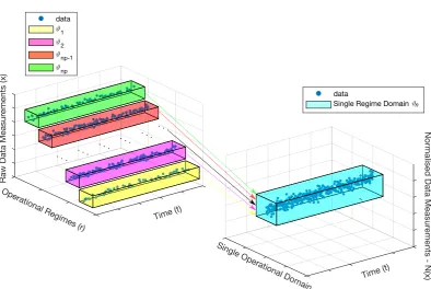
3.3 A sample demonstration of z-scores in a normal distribution . 105 3.4 Normalisation of Multidimensional Data . . . 107

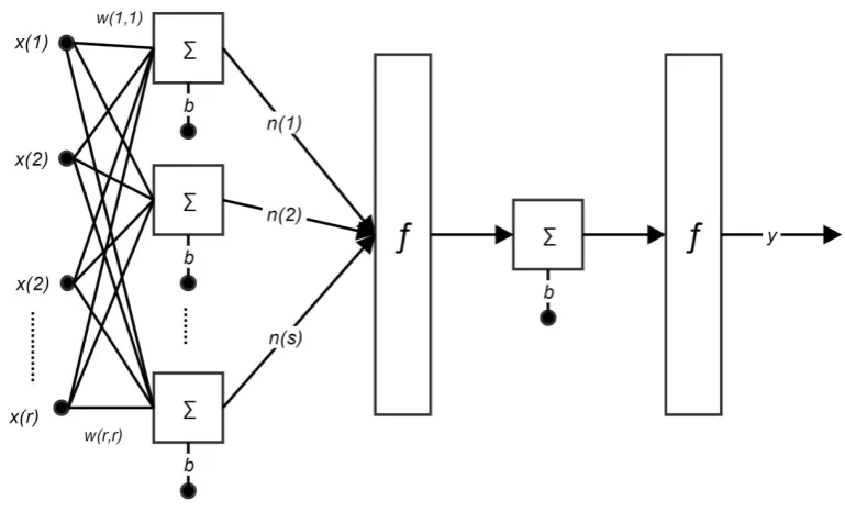
3.5 Feed-forward neural network with multidimensional input data and HI output . . . 113

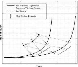
3.6 Similarity Methodology . . . 120

3.7 RUL Estimation . . . 121

4.1 A simplified diagram of an engine simulation modelled in C-MAPSS . . . 128

(10)

4.3 Flowchart representing data processing and multistep ahead

re-maining useful life calculation . . . 133

4.4 Raw Data Characteristics . . . 134

4.5 Sensor 11 - Static pressure at HPC outlet . . . 135

4.6 Sensor 11 - Static pressure at HPC outlet (y-axis limited) . . 136

4.7 Operational settings in different regimes . . . 137

4.8 Sensor 1 with constant values at each regime domain . . . 138

4.9 Clustered Regimes for Sensor 11 - Static pressure at HPC outlet 139 4.10 Normalised Sensors . . . 140

4.11 Useful sensors in all training trajectories . . . 141

4.12 Non-Useful sensors in all training trajectories . . . 141

4.13 Useful Normalised Sensors . . . 142

4.14 Adjusted Trajectory and HI . . . 144

4.15 Alternative Fitting Functions . . . 144

4.16 Neural Network Learning Stage . . . 146

4.17 Neural Network validation with the same input . . . 147

4.18 Neural Network estimation with a different input . . . 148

4.19 Neural Network Library Results . . . 149

4.20 Moving Average Applied in Network Library Estimations . . . 151

4.21 Comparison of Full and Interrupted Data . . . 152

4.22 Pairwise Distance Calculation . . . 155

4.23 Minimum Pairwise Distance Position and Best Matching Location155 4.24 Top similarities and RUL calculation . . . 156

4.25 Test trajectories resulting in a wide range of RUL estimations 157 4.26 HI Estimation from a Network Trained using a Synthetic Target 160 4.27 Synthetic Raw Data with a Linear Decrease . . . 163

4.28 Network Estimations for Synthetic Data . . . 164

(11)

5.1 Comparison of True and Predicted RULs . . . 175

5.2 Demonstration of density estimations of predicted RULs . . . 176

5.3 Comparison of Absolute Error and Unit Test Length for SD#1 179

5.4 Risky positions with respect to the data fluctuation . . . 179

5.5 RUL calculation for Unit #421 . . . 180

5.6 RUL calculation for Unit #3 . . . 180

5.7 Comparison of Absolute Error and Scoring Function for

Sec-ondary Dataset #1 . . . 181

5.8 Demonstration of density estimation of predicted RULs . . . . 182

5.9 Comparison of Absolute Error and Unit Length for Secondary

Dataset #12 . . . 184

5.10 Comparison of Absolute Error and Scoring Function for

Sec-ondary Dataset #12 . . . 184

5.11 Top Matching Similarities and RUL calculation for Dataset

#12, Trajectory Unit #421 . . . 185

5.12 Top Matching Similarities and RUL calculation for Dataset

#12, Trajectory Unit #3 . . . 185

A.1 Clustered Regimes for Raw Sensors . . . 239

(12)

Acknowledgments

I would like to thank my supervisors, Dr Jeffrey Jones and Dr Jane Marshall,

for their kind support and guidance throughout my research. Their supervision

and advice are of inestimable value for my study.

I want to express my thanks to my thesis examiners: Dr Faris Elasha

and Dr James Marco for their kind comments and corrections in my thesis. I

appreciate them taking the time out to examine my thesis.

I would like to thank Dr Kai Goebel and the Prognostics Center of

Excellence of NASA Ames Research Center for their support of my work.

Their hospitality during my research visit is most gratefully acknowledged.

I would also like to thank my department, research fellows, advisors

and collaborators; their discussion, ideas, and feedback have been absolutely

invaluable.

I would like to thank the people of Turkey for providing the government

scholarship which allowed me the opportunity to fulfil my dreams.

Finally, I would especially like to thank my amazing family for their

love, support, and encouragement. In particular, I would like to thank my

wonderful wife “Aysenur Bektas” who has made countless sacrifices to help us

get to this point and my little son “Yavuz Selim” who always gave his father

extra motivation to finish this thesis as soon as possible.

To all those cited by name here and the many more I could not mention

by their name, I will forever owe you this achievement.

Thank you all most sincerely - Hepinize en i¸cten dileklerimle te¸sekk¨ur

(13)

Declarations

I hereby declare that this thesis is my own work and effort and that it has not

been submitted anywhere for any award. Where other sources of information

have been used, they have been acknowledged.

I undertake not to quote or make use of any information from this thesis

without making acknowledgement to the author. I further undertake to allow

no-one else to use this thesis while it is in my care.

The material is based upon work supported in part by NASA under

award NNX12AK33A with the Universities Space Research Association. Any

opinions, findings, and conclusions or recommendations expressed in this

ma-terial are those of the author and do not necessarily reflect the views of the

National Aeronautics and Space Administration.

Parts of this thesis have been published by the author:

1. Poster presentation at WMG Research and Innovation Conference on

the 10th and 11th July 2014. A Framework for Performance Metrics

of Rotating Machinery Prognostics within Maintenance Free Operation

Period -Oguz Bektas

2. Conference Proceeding in The Twelfth International Conference on

Con-dition Monitoring and Machinery Failure Prevention Technologies CM2015

(14)

Engines -Oguz Bektas & Jeffrey Jones

3. Technical Presentation at WMG Research and Innovation Conference on

the 30th June and 11th July 2015. Narx Model in Gas Turbine

Prognos-tics -Oguz Bektas

4. Conference Proceeding in Third European Conference of the PHM

So-ciety - PHME16. NARX Time Series Model for Remaining Useful Life

Estimation of Gas Turbine Engines -Oguz Bektas & Jeffrey Jones

5. A journal article in Journal of Failure Analysis and Prevention. “

Reduc-ing Dimensionality of Multi-regime Data for Failure Prognostics - Oguz

Bektas, Amjad Alfudail, Jeffrey A. Jones

(15)

Abstract

The field of Prognostics and Health Management is becoming ever more important in the modern maintenance era, with advanced techniques of automa-tion and mechanisaautoma-tion becoming increasingly prevalent. Prognostic technology has promising abilities to forecast remaining useful life and likely future circumstances of complex systems. However, the evolution of data processing and its critical impact on remaining useful life predictions continually demand increasing development so as to meet higher performance levels. There is often a gap between the adequacy of prognostic pre-processing and the prediction methods. One way to reduce this gap would be to design an adaptive data processing method that can filter multidimen-sional condition monitoring data by incorporating useful information from multiple data sources.

Due to the incomplete understanding on the multi-dimensional failure mech-anisms and the collaboration between data sources, current prognostic methods lack the ability to deal effectively with complicated interdependency, multidimensional condition monitoring information and noisy data. Further conventional methods are unable to deal with these efficiently. The methodology proposed in this research handles these deficiencies by introducing a prognostic framework that allows the effective use of monitoring data from different resources to predict the lifetime of systems. The methodology presents a feed-forward neural network filtering approach for trajectory similarity based remaining useful life predictions. The extraction of health indicators is applied as a type of dynamic filtering, in which the time se-ries having full operational conditions are used to train a neural network mapping between raw training inputs and a health indicator output. This trained network function is evaluated by repeating condition monitoring information from multiple data subsets. After the network filtering, the training trajectories are used as base-lines to predict the future behaviours of test trajectories. The similarity between these data subsets compares the relationship between the historical performance de-terioration of a system’s prior operating period with a similar system’s degradation behaviour.

The proposed prognostic technique, together with dynamic data filtering and remaining useful estimation, holds the promise of increased prediction performance levels. The presented methodology was tested using the PHM08 data challenge provided by the Prognostics Centre of Excellence at NASA Ames Research Centre, and it achieved the overall leading score in the published literature.

(16)

Symbols

The following list contains the symbols most frequently used in this thesis. References to sections are given at the beginning and then the symbols are defined.

Section 2.1 & 2.2

Ω Dimensions space

Ψ Dimension levels space

Cb Multidimensional data set

D List of dimensions

L List of regime levels

R Set of multidimensional data

x Multidimensional data

H Health Measure

∆θ Life distance

ε Noise

pG(ε) Gaussian Noise

µ Mean

σ Standard Deviation

SN R Signal to Noise Ratio

Psignal Power of signal

Pnoise Power of noise

X Variable of RUL

t Time index

Z Preceding condition profile

Rt Survival function

θt History of operational profiles

P H Prognostic horizon

EOP End of prediction

Section 2.3

a Crack length

∆K Range of stress intensity factor

q Training trajectory

p Test Trajectory

fs State transition function

fm Measurement function

¨

x Damage State

¨

p Model parameters

˙

ε Process noise

¨

(17)

Fs State evolution matrix

Fm Measurement matrix

P Autoregressive model order

Q Moving average model order

φ Auto-regressive term

Θ Moving average term

y Target variable

β Coefficients

d Regime

h Health index

e(t) Efficiency

H Overall health index

w Weight

b Bias

M ANN model

H Hessian matrix

Section 2.4

e Error

AE Absolute error

M AE Mean absolute error

AB Average bias

M SE Mean square error

F P False positive rate

F N False negative rate

M AP E Mean absolute percentage error

M AD Mean absolute deviation from

the sample median

M dAD Median absolute deviation from

the sample median

s Score function

Section 3

Ω Multidimensional space

T Operational trajectory

r Regimes (operating conditions)

x Raw condition monitoring data

n Number of time series points

θ(t) Number of unique time index variables

θ(r) Number of unique regimes

np Number of regimes

lr Lower regime domain limits

ur Upper regime domain limits

ϑr Regime domain

wp Noise and measurement

uncer-tainties at regime, p

Hp Health information at regime, p

tcurrent Time stamp of the current

mea-surement index

tend Ending time stamp

ttest Time index of the test instance

ttraining Time index of the training

(run-to-failure) instance

(18)

d Initial wear level

a, b Degradation model parameters

ns Number of sensors

fN N Neural network function

y Neural network output (target)

N(x) Normalised data

xr _{Raw data at regime} _r

σr _{Standard deviation of regime} _r

µr Mean of regime r

c Cluster variable

x(c) Raw data at cluster c

σ(c) Standard deviation of cluster c

µ(c) Mean of cluster c

ˆ

x(c) Normalised data at cluster c

s Moving average

f(x(t)) Feed forward neural network function

wi Fixed real-valued weights

L(i) Neural network library

l Number of trained network

functions

d Euclidean distance

ntr Length of the base curve

(train-ing trajectory)

nte Length of test trajectory

M n Stored pairwise distances

Lte,tr Location of the best-matching

part at the training baseline

Section 4

(19)

Abbreviations

AB Average Bias

AN N Artificial Neural Network

ARM A Auto-Regressive Moving-Average

AT T F Actual Time to Failure

BR Bayesian regularisation

CBM Condition Based Maintenance

C−M AP SS Commercial Modular Aero-Propulsion System Simulation

ES Expert Systems

EOP End of Prediction

ET T F Estimated Time to Failure

F EA Finite Element Analysis

F L Fuzzy Logic

F N False Negative Rate

F P False Positive Rate

HI Health Indicator

HP C High Pressure Compressor

HP T High Pressure Turbine

HM M Hidden Markov Model

IGBT Insulated Gate Bipolar Transistors

KbM Knowledge-based Models

(20)

LP C Low Pressure Compressor

LP T Low Pressure Turbine

LQE Linear Quadratic Estimation

M A Moving Average

M AD Mean Absolute Deviation from the Sample Median

M dAD Median Absolute Deviation from the Sample Median

M AE Mean Absolute Error

M AP E Mean Absolute Percentage Error

M LP Multi-Layer Perceptron

M RO Maintenance, Repair, and Operations

M SE Mean Square Error

N N Neural Network

N F LT No Free Lunch Theorem

P bM Physics-based Models

P CA Principal Component Analysis

P CoE Prognostics Center of Excellence

P DF Probability Density Function

P F Particle filtering

P H Prognostic Horizon

P HM Prognostics and Health Management

P M Preventive Maintenance

RBF N Radial Basis Function Networks

RN N Recurrent Neural Network

RU L Remaining Useful Life

SD Secondary Dataset

SM C Sequential Monte Carlo

(21)

Chapter 1 Introduction

The focus of reliable systems community is on the basic principles of system

failures to explain how complex systems age and fail. Over the last decade,

Prognostics and Health Management (PHM) has been an emerging discipline

as a responding point to this focus, and it has established a connection with

failure mechanisms and system life-cycle management (Uckun et al., 2008).

PHM aims to maximise operational availability and safety by incorporating

functions of condition monitoring, prognostics, state assessment, diagnostics

and failure progression (Sheppard et al., 2008). Due to the constantly

increas-ing interest in PHM technologies, which has received great attention from the

industry at all levels, there has been a significant change in attitude towards

these functions.

As a steadily growing subject in PHM applications, prognostics are a

particularly well-known practice in a wide variety of applications (Lee et al.,

2014). The term “prognostics” in the context of PHM field refers to the

es-timation of a time at which a system (or a component) is at the end of its

useful life point and will no longer perform its desired functional requirements

(Saxena et al., 2014). Therefore, prognostic methods are mainly focused on

(22)

main-tenance decision making process (Sandborn and Wilkinson, 2007). Within the

last decade, these methods have advanced expertise in various disciplines and

an overall understanding of the predictions for health management has

sub-stantially improved. Many breakthroughs in prognostics and their ability to

predict RUL for maintenance purposes can be found in various areas, notably

in advanced engineering systems such as, gearboxes (Elasha et al., 2014a,c,

2015b,c, 2017), batteries (Pastor-Fern´andez et al., 2016; Saha et al., 2009;

Goebel et al., 2008a; Rezvani et al., 2011), actuators (Byington et al., 2004b),

fuel cells (Morando et al., 2013), turbofan engines (Wang et al., 2008; Heimes,

2008; Peel, 2008) and even NASA‘s launch vehicles and spacecraft systems

(Luchinsky et al., 2007).

Prognostic technology has also been used to design platforms with

pre-diction capacity as an integral feature of the overall system architecture (Uckun

et al., 2008), such as the Joint Strike Fighter Programme and the Future

Com-bat Systems Programme (Hess et al., 2004; Barton, 2007). As the technology

develops further, prognostics continue to play a prominent role in the evolution

of such complex systems. Introducing prognostic development to the earliest

stages of complex system design can highlight elements requiring

reconsider-ation earlier in the design stage and allows the process of testing, validating,

and refining to provide a higher quality design (Kramer and Tumer, 2009).

Many advanced modelling techniques exist for system design and significant

research have been related to the predictive capabilities for future operations,

and resulted in the development of notable prognostic applications. The

ma-jority of these applications concentrate on imposing alternative strategies for

maintenance, and have led to a huge and diverse literature on machinery

prog-nostics with a considerable number of papers, substantial theories and practical

(23)

1.1 Motivation

Today, many sophisticated sensors and computerised components are

capa-ble of delivering system’s performance data to prognostics that can

contin-uously track health degradation and extrapolate the temporal behaviour of

system’s health to predict risks of unacceptable performance over time as well

as synchronising necessary maintenance actions with the overall operation of

the system (Lee et al., 2006). Since the key point in maintenance actions is

the involvement of all operation-related activities (BSI, 1993), the prognostic

applications are directly related to the development of prediction-based

main-tenance actions required to keep systems at a desired level of mainmain-tenance

with minimum operational cost. The structure of maintenance, accordingly, is

highly interrelated with prognostics to reduce maintenance expenses. To gain

an appreciation for prognostic technology and amounts of maintenance

expen-diture, the global airlines market can be considered an illustrative example. In

2014, the worldwide airliner spending on maintenance, repair, and operations

(MRO) accounted for $62.1 billion, in which engine maintenance was about

40% of the total cost (IATA, 2011). Although the size of the MRO market

is expected to reach $90 billion in 2024, it is estimated that the developing

trends in such areas as prognostics, innovations and technologies will reduce

MRO costs by 15 to 20%, and predictive maintenance strategies are expected

to increase airliner availability by up to 35% (IATA, 2011).

As the predictive maintenance strategies develop, the ability to find

solutions to key challenges have become a crucial push towards developing

models that apply performance in maintenance. In this context, data

pro-cessing for maintenance decision making can be regarded a major step in a

successful maintenance programme (Tsang et al., 1999; Jardine et al., 2006a).

In order to avoid unnecessary maintenance tasks, data processing analyses

(24)

re-quired (Lee et al., 2014). However, unless the uncertainties in the predictions

are also considered, data processing may not be a sufficiently practical step

for decision makers to justify the need for prognostic actions (Goebel et al.,

2013). Since it is very unlikely to attempt to estimate the operating and

environmental conditions under which a given system operates, a systematic

framework for data processing is necessary to account for the uncertainties in

prognostics (Sankararaman and Goebel, 2015). Data processing should

han-dle and analyse the condition monitoring data for a better understanding and

interpretation of the system’s damage propagation, which characterises how

the damage is expected to grow in upcoming operational and environmental

conditions, along with any other effects that might have an impact on damage

(Goebel et al., 2013).

1.2 Problem Statement

Recent technological advances have resulted in increasingly complex systems

that pose considerable challenges in terms of successful operations and use over

their life cycles (Venkatasubramanian, 2005). Ensuring safety and performance

in complex and safety-critical systems is a major problem to be tackled, and

above all, complexity is one most prominent issue that must be addressed to

make theoretical models applicable to real-life applications (Boussif, 2016). A

complex engineering system is defined as a group of interrelated, interacting,

and/ or interdependent components (constituents) forming a complex whole

(Jamshidi, 2008).

Condition monitoring of such complex systems is usually based on

var-ious sensors of components to receive information on the system health status

and recognise any potential problems at an early stage so that corrective

(25)

interpretation of sensor data from multiple elements is often a challenging

as-pect due to complicated interdependencies between monitored data and actual

system conditions (G¨unel et al., 2013).

As a result of operational conditions and regimes, some complex

sys-tem works under different superimposed operational margins at any given time

instant and the wearing process of such systems is not usually deterministic,

and commonly not one-dimensional (Saxena et al., 2008b). These

multidimen-sional and noisy data streams are measured from a large number of monitoring

channels from a population of similar components such as the operational or

environmental conditions, direct and indirect measurements that are

poten-tially related to the damage progress (Uckun et al., 2008). Therefore, a simple

model is mostly unable to present the wearing phenomena and one should

con-sider a more advanced decision-making process for the condition monitoring

data in multidimensional form (Cempel, 2009).

While the literature has recognised the importance of the multiple axes

of information and multidimensional data, there is still a lack of analysis in

such data, leaving the analysts with yet more information and data to process

through the complex systems (Tumer and Huff, 2003). This can be attributed

to two fundamental issues:

• Incomplete information on the multi-dimensional mechanisms failure and fault modes;

• Lack of collaboration between different but similar data sources

When a prognostic model planned and tested under controlled

experi-ments, it has to face the challenges brought up by the complexity of real-world

systems (Wang, 2010). The models should reduce the future uncertainty of

operations according to the needs of system itself, and limitations of

(26)

prognostic algorithm for a successful and practical implementation in complex

systems depends on understanding of the challenges associated with the type

of applications (Zaidan et al., 2013). Therefore, the majority of prognostic

researches to date has been mostly disparate, theoretical and restricted to a

small number of cases, and there are few published examples of full prognostic

frameworks being applied in the field of complex systems where the

moni-tored condition data are exposed to a range of dynamic operating conditions

(Sikorska et al., 2011).

1.3 Research Question and Hypotheses

The key element to design prognostics for such complex systems is the data

pro-cessing for conditioning and feature extraction of acquired multidimensional

data. For RUL estimations, data processing capabilities are of greater

signif-icance for design and implementation point of view (Saxena et al., 2008a). If

condition monitoring data is not available sufficiently, the prognostic

require-ments cannot be met (Uckun et al., 2008). One way to satisfy the prognostic

requirements is to perform a data collaboration effort distributed across

mul-tiple suppliers, rather than using separate and self-contained sources.

Collab-oration, from this perspective, is the act of working together with one or more

sides in order to achieve the objective of higher accuracy (Soukhanov, 2001);

when used in intelligence-intensive activities, this may lead to increased and

improved results (Moyle, 2009).

Additionally, data processing can be understood as the conversion of

multidimensional and complex monitoring data to meaningful information for

RUL estimation. Because the effort needed to filter prognostic parameters

from multiple data can quickly make the prognostic approach applicable for

(27)

optimal, or near-optimal, filtering is very promising for RUL estimations.

The literature shows that because of the lack of understanding on the

multi-dimensional failure mechanisms and incomplete collaboration between

different but similar data sources, current prognostic methods are unable to

deal effectively with complicated interdependency (G¨unel et al., 2013),

multi-dimensional data (Saxena et al., 2008b) and noisy data (Uckun et al., 2008).

The traditional pre-processing models lack the ability to address this efficiently.

The method proposed in this research handles these issues by introducing an

adaptive data filtering model for RUL estimation.

The main focus in the research is to make an original contribution to

the development of prognostics by considering data filtering requirements on

multiple data resources. The point at issue is the modelling of such a

concep-tual prognostic framework to overcome the challenges presented by different

datasets and to increase prediction performance. The model should be based

on adaptation of complicated prognostic filtering algorithms for different

exter-nal input resources and satisfying the generic demands on the performance of

RUL predictions by using alternative trained functions. In this respective, an

effective method is necessary to approximate any filtering function arbitrarily

well.

In this work, the intention to use such an adaptive filtering function

is to visualise information from different but similar data sources, and get

this information to the right place, in the right arrangement, and in good

time to use it in making effective predictions. Then, a prognostic prediction

method can be swamped with data from multiple sources and investigate data

filtering and processing techniques, with the ultimate goal of improving RUL

predictions.

Research Question

(28)

”How can an adaptive data filtering model be designed as a part of

multi-step ahead remaining useful life predictions? ”

Research Aim

The aim of this research is to study the possibility of developing a prognostic

and health management prediction approach to complex machinery systems

under dynamic operating regimes. This prediction is based on the systematic

monitoring of multidimensional data and the filtered available information,

and it is in line with adaptable stages consisting of data processing and

multi-step ahead predictions. Therefore, the research aims to develop a multifaceted

prognostic approach that integrates data filtering and RUL estimation to

en-hance the prediction results and to increase the applicability of prognostics

and health management in machinery applications under a set of operational

cases with multi-regime operating conditions.

Research Objectives

The research has following key objectives that will help to satisfy the

above-mentioned issues and address the current gap indicated by the research

ques-tion.

• To develop an understanding of emerging concepts of prognostic use in maintenance

• To design an adaptive prognostic model that can process filtering and prediction modes

(29)

• To develop a merging process between data qualification and RUL esti-mation

• To increase the performance of RUL estimations and provide more

de-tailed results in terms of maintenance planning

• To reduce excessive RUL prediction error rates for critical cases

• To minimise the gap between false positive or negative error rates of life-time predictions

1.4 Significance and Contribution

The significance of this study can be found in the sense that it can introduce

a novel perspective to data filtering and prognostics accuracy by considering

multi-dimensional condition monitoring data from complex systems. A

con-sideration of operational requirements in terms of multiple data employment

has improved the prediction performance of prognostics. An adaptive

prog-nostic method is designed to introduce a sequential process from training to

prediction. A neural network-based data training function is presented to map

between a set of raw monitoring inputs and a set of targets. Then, external

datasets are applied to this function to allow for an adjustment from their raw

scales to a notionally common target scale. This allows for the fact that

mul-tiple data sources can be filtered separately and be used for RUL estimations.

The contribution of this study, as a response to the formulated research

question, is the introduction of a data-driven filtering process (feed-forward

neural network) into collaborative RULs (trajectory similarity-based

prognos-tics). In particular, the research investigates how pre-processing methods

af-fect algorithm performance. The algorithm will be tested by PHM08 data

(30)

1.5 Thesis Organisation

This thesis is composed of six chapters. The organisation of thesis is as follows:

Chapter 2reviews the progress of the current literature and gives the state-of-art on current prognostic applications as well as the various sources

and methods applied in complex system domains.

Chapter 3 includes the methodology sections. This chapter provides the details of the multi-regime normalisation, data filtering and RUL

predic-tion frameworks. A feed-forward dynamic network relating to the raw input

time series with a target vector is introduced. Then, the similarity-based

fore-casting setup is summarised.

Chapter 4applies the presented method to different case studies which are then used as examples of how to gain a better understanding of the risks

posed by various conditions. Case studies contribute to more focused analyses

which, in the context of damage, demonstrate the effectiveness of prognostic

methods and metrics, and identify risks in multi-step ahead projections.

Chapter 5 brings forward the analysis, performance evaluation and validation of the model, as based on true RUL parameters. The chapter also

deals with the issues of critical assessment of this study, contribution to

knowl-edge, and a comparison of this model with rival ones.

(31)

Chapter 2 Background and Literature

Survey

Maintenance has witnessed substantial changes, perhaps more so than any

other discipline in the industry as a direct result of an increase in the

vari-ety and quantity of complex systems requiring novel practices and progressive

views (Moubray, 1997). Due to the increasing awareness of high plant

avail-ability and reliavail-ability, maintenance strategies have been going through a stage

where there is a necessity to respond the rapidly changing expectations. There

is a significant risk that complex systems and their related interfaces would

not be satisfied by classic breakdown repairs; therefore, various approaches

in maintenance applications have been defined in an attempt to meet their

increasing requirements (Jardine and Tsang, 2013).

A classification of maintenance is shown in Table 2.1. Simply, the

poli-cies are divided into unplanned and planned categories according to the

histor-ical perspective of maintenance. These types are related to how a user would

like to approach repair procedures. Determination of the optimum schedule

for performing maintenance has been a long-standing challenge. Maintenance

(32)

Table 2.1: Classification of Maintenance (BSI, 1993; Jones, 2010)

Unplanned Maintenance: or “run to failure”, is an option of “do nothing until it breaks”

Corrective

Maintenance It is carried out after a failure has occurred Emergency

Maintenance

EM is required where immediate action is necessary to avoid serious consequences

Planned Maintenance: carried out and organised with forethought

Preventative Maintenance

PM performed at predetermined intervals. It aims to reduce the probability of failure.

Scheduled Maintenance

It attempts to forestall breakdown by operating on a predetermined interval of time

Condition-Based Maintenance

CM is initiated as a result of condition monitoring knowledge. It seeks to determine actual operating conditions

maintenance, to preventive maintenance (PM) schemes, and then to

condition-based maintenance (CBM) (Heng et al., 2009). Breakdown maintenance was

the earliest attitude taken, including the repair or replacement of equipment

when a failure occurs (Misra, 2008). This type of basic approach shifted

to-wards PM in order to prevent unscheduled downtime and avoid catastrophic

failures. However, each maintenance type has still its own unique

advan-tages that make each desirable for specific needs. For example, until the most

spectacular changes that occurred in maintenance after World War II (Brown

and Sondalini, 2014), corrective maintenance had been the only option for a

maintainer to fix or replace an item; that is after a failure had occurred.

Nev-ertheless, corrective maintenance is still in use for simple components in which

the failure consequences are less critical. Moreover, no matter how extensive a

(33)

may fail and corrective maintenance become necessary (Sheut and Krajewski,

1994). On the other hand, changing customer requirements demand planned

maintenance designs at all levels. From the 1950s, mechanisation and

automa-tion of systems have arisen due to an increasing intolerance of downtime and

labour costs, with the first planned maintenance practices introduced in the

form of preventive maintenance to avoid catastrophic failures and emergency

shutdowns (Heng, 2009).

In the case of PM, maintenance is carried out on a regular basis to

reduce the failure rate or performance decrease of given piece of equipment

(BSI, 1993). Preventive actions involve fixed scheduled servicing, inspections,

and repairs to reduce failures and costs. In such a procedure, maintenance

is considered where inspections and overhauls take place at different time

in-tervals without seriously considering the condition of a given system’s health

(Badıa et al., 2002).

Bazovsky (1961) laid the groundwork for the application of

mathemat-ical optimisation methods in PM plans and Jardine (1973) pioneered decision

models for assignment of optimal replacement and/or repair intervals by

inves-tigating historical breakdown measures and cost implications. In subsequent

years, Lee and Rosenblatt (1987) analysed the use of machine inspection in PM

for restoration purposes of economical manufacturing quantity, and Groenevelt

et al. (1992) studied the role of PM in an unreliable production system with a

constant failure rate and randomly distributed repair times. Other studies have

also shown that PM strategies can be an effective way to extend the lifetime of

several randomly failing production units and reduce operational costs (Barlow

and Proschan, 1996; Nakagawa, 1981; Nakagawa and Yasui, 1991). Under the

assumption of non-negligible maintenance restoration times, all these studies

addressed the use of planned maintenance that is regularly performed on a

(34)

increas-ing system complexity, these scheduled maintenance policies have financial

and safety implications that may result in labour-intensive and unnecessary

maintenance actions that can be associated with over-maintaining. While PM

strategies are robust enough to continue earlier and relatively simple routine

maintenance tasks to reduce component damage, they may have shortcomings

when dealing with catastrophic failures in complex systems. PM approach

can be costly when it is, or needs to be, performed frequently (Bohlin et al.,

2010), and fixed scheduled maintenance policies are not considered functional

by most practitioners (Kelly, 1989). This is why, it is necessary to invest in

monitoring efforts to maintain the correct item at the right time. Dynamic

planning using malfunction signs is required to reduce unpredictable events

and unnecessary maintenance tasks.

In recent times, the performance of PM has started to be questioned.

Wood (1999) and Moubray (1997) defended the idea that scheduled and

time-based PM often fails to make best use of the remaining service life; on many

occasions, units are replaced despite the fact that they have many hours of

RUL. The fixed repair intervals required by PM tasks waste a considerable

amount of resources (Tsang, 1995), such that systems or units are often

un-reasonably maintained (Ellis and Byron, 2008). These queries resulted in the

subdivision of CBM.

A properly and effectively established CBM programme can notably

decrease maintenance costs by dropping unnecessarily scheduled preventive

maintenance actions (Jardine et al., 2006a). CBM is similar to PM in the

sense that it aims to prevent abnormality in advance of an incident, but it

differs from the fixed time-oriented approach of scheduled maintenance (Shin

and Jun, 2015). Hence, CBM offers an alternative to PM considerations of

simple age-related failure modes.

(35)

at-tention from maintenance service providers and end users who require higher

planned maintenance performance, and the reduction of unnecessary

inspec-tions (Chen et al., 2012; Ahmad and Kamaruddin, 2012; Gulati and Mackey,

2003). Use of CBM in industry, therefore, has been reported to be one of the

most substantial ways to decrease maintenance budgets (Bengtsson, 2004), and

have thus seen a considerable increase in their uptake over time. For example,

in 1981, domestic plants in the United States had spent more than$600 billion

in maintaining critical systems; by 1991, this cost increased to more than$800

billion, and exceeded$1.2 Trillion in 2000 (PlantServices, 2004). Considering

that the cost of ineffective maintenance constitutes around one-third of the

total maintenance cost, and there is a similar trend in many other countries,

there is a clear and immediate need to continuously progress and improve

cur-rent maintenance strategies (Heng et al., 2009). As a response to this need,

CBM allows maintenance service providers to avoid the inevitability of

high-cost maintenance due to the elimination of redundant maintenance activities

(Shin and Jun, 2015).

2.1 Condition Based Maintenance

Condition-Based Maintenance is a programme recommending maintenance

ac-tions based on condition monitoring data (Raheja et al., 2000); it attempts to

avoid redundant tasks by taking repair actions only when there is evidence of

unexpected operational issues (Jardine et al., 2006a). Certain signs, condition

changes, or malfunction indications can precede the vast majority of machine

failures (Pusey, 1999; Heinz P. Bloch, 2012), and maintenance actions based

on monitoring can be taken prior to a severe performance reduction in a given

system, with condition-based monitoring offering the ability of yielding

(36)

According to Horner et al. (1997), the optimal time period for

per-forming maintenance could be decided by the actual monitoring of a given

system, and its subcomponents or units, and the condition monitoring

assess-ment could vary from basic visual checks to detailed automatic inspections.

Considering the continuous data related to the operational condition of

criti-cal systems, Knapp and Wang (1992) argued that CBM aims to minimise the

cost of repairs, and Knapp et al. (2000) noted that condition monitoring can

provide adequate warnings as to pending failures, which would thus allow for

more detailed planned maintenance actions as based on system degradation.

On the other hand, as stated by Ellis and Byron (2008), CBM in some

instances may not be cost-effective or sufficient data may not exist to justify

intervention. Raheja et al. (2006) also claimed that some current CBM

ap-proaches are extremely specific and a common structure for CBM is missing,

so that each domain has its own understanding that may not be well-suited for

the requirements of other applications. Although CBM may not be applicable

to all maintenance systems, it could be applied in instances where modules

of condition-monitoring are available and are well-integrated (Horner et al.,

1997)

Such typical modules of effective CBM implementation include the

stages of data acquisition (information collecting), data processing

(informa-tion handling) and maintenance decision-making (see Figure 2.1). These three

key elements provide the necessary conditional information on which the

main-tenance process can be based, and help to avoid unnecessary mainmain-tenance

op-erations. The data acquisition and processing modules in a CBM programme

are critical pre-processing stages that present and process monitoring data to

produce the information useful to the diagnostic and prognostic stages. After

the raw condition monitoring data is processed, organised and restructured,

(37)

identification, while prognostics deal with the prediction of the future lifetime

of a system over a fixed time horizon (Brotherton et al., 2000). These lifetime

estimation applications are key enablers of the CBM strategy (Byington et al.,

2008), and have significant value within complex system operations in terms

of maintenance scheduling thus the reduction of maintenance downtime and

costs (Brotherton et al., 2000).

Data Acquisition

• Event Data

• Condition monitoring data

Data Processing

• Signal processing

• Feature extraction & selection

Maintenance Decision

Making

• Diagnostics

• Prognostics

Figure 2.1: Major Steps in CBM

CBM objectives are designed to determine the condition and the

re-maining life of in-service equipment. Diagnostics and/or prognostics can be

effectively used according to these objectives, and applied when developing

the decision-making stage of complex maintenance applications (Heng et al.,

2009). They are considered as significant procedures effecting a substantial

shift in the current manner of technology that can push the boundary of

sys-tems health management (Elattar et al., 2016).

2.1.1 Data Acquisition

In the data acquisition stage, useful information is collected and stored from

target physical assets in order to monitor the condition of systems, diagnose

faults, and predict the remaining lifetime of assets (Tran and Yang, 2012).

In parallel with the increasing development of advanced computer and sensor

(38)

expen-sive technologies that could implement data for CBM in a more affordable and

feasible way (Jardine et al., 2006a).

Data acquisition for a CBM programme is mainly supported by

condition-monitoring data. For a complex mechanical system, condition condition-monitoring

in-formation can be very diverse; superficially, it can constitute temperature,

acoustic, oil analysis, environment moisture or weather data, etc. Condition

monitoring of such systems in operation is generally multidimensional

(Cem-pel, 2003). The analysis and extraction of useful information from

multidimen-sional data is inevitably based on high-performance computing capabilities of

data processing (Baurle and Gaffney, 2008).

Although condition monitoring could provide sufficient information for

the development of data processing, there is still the requirement to collect

common datasets and a mutual comparison to validate the methods introduced

by different researchers. However, the nature of data acquisition has its own

challenges in terms of the availability of condition monitoring data (Eker et al.,

2012). To start the acquisition of raw monitoring data for effective lifetime

estimations, the first major issue is to find available data sources. A common

database is an important aspect for life estimation applications of maintenance

decision making (Kans and Ingwald, 2008). Considering that such a database

includes information from several but similar engineering domains, it can form

the basis for the stage of data acquisition and required actions (Sim˜oes et al.,

2011).

Use of the common database practice allows for the comparison of

cur-rent applications and potential areas of improvement with regard to other

re-searches in the literature (Bask et al., 2008), and since this type of a database

can provide easy access to relevant data, it can demonstrate the detection of

deviations at an early stage (Sim˜oes et al., 2011). However, Saxena et al.

(39)

a deficiency of common run-to-failure data sets, and that real-world data in

most cases includes fault signs for an increasing degradation but no or little

data capture for fault progress until failure. There have been synthetic data

generating methods that can closely match the characteristics of raw data

such as Eklund (2006); Zaidan et al. (2013); Bektas and Jones (2015) but

these methods were developed for individual cases and the common data sets

through which researchers can compare their approaches are required for an

effective data acquisition stage in CBM.

2.1.2 Data Processing

A major issue confronting condition monitoring is ability to handle the

col-lected data in terms of measurable machinery conditions. Data processing is

the most critical stage in CBM because it is not always clear during the

col-lection and manipulation of raw data from different sensors when meaningful

information useful to lifetime estimations is being produced (Vatani, 2013).

Condition monitoring data collected from the data acquisition stage

is versatile and falls into various categories such as value type (single value

collected at a specific time epoch ), waveform type (time series of a condition

monitoring variable) and multidimension type (multidimensional time series

acquired from multiple operating conditions) (Jardine et al., 2006b) .

In the case of complex systems under dynamic operating regimes, special

attention is given to multidimension type data as it requires more processing

and many techniques have been developed for its analysis and interpretation.

Raw multidimensional data acquired from sensors providing information under

multiple operating conditions are almost always processed before it is used for

further analysis.

A typical complex system is made of different interacting components

(40)

individ-ual components, system predictability is limited, and the responses do not

scale linearly (Bar-Yam, 2003). Additionally, the technological advancements

have resulted in easy and efficient generation of data sets, most of which are

multidimensional and/or multivariate (Seo, 2005).

A multidimensional database is composed of sets of vectors on

rela-tional elements constructed from hierarchies of dimension levels (Vassiliadis,

1998). Considering Ωas the space of all dimensions andΨas the space of all dimension levels, for each dimension D there exist a set of regime levels and

there is a set of values belonging to it. Accordingly, a basic multidimensional

data set,Cb, can be defined as a 3-tuple <Db,Lb,Rb > (Vassiliadis, 1998),

where

Db=< D1, D2,· · ·Dn, M > (2.1)

is a list of dimensions (Di, M ∈Ω) andM is a dimension that represents

the measure of Cb.

Lb=< DLb1, DLb2,· · ·DLbn,∗M L > (2.2)

is a list of regime levels (DLbi,∗M L ∈ Ψ). M L is the multi-valued

dimension level of the measure of Cb. Rb is a set of cell data and formed of

x= [x1, x2,· · · , xn] (2.3)

Having specified this cell data, there is a possibility to assess the system

breakdown time,θb, by using the life dependence of observed sensor readings,

R, in terms of a function of some simplified health measure,H (Cempel, 2003).

H= t

tb

(41)

where t is the current system life time and tb is the anticipated breakdown

time. A single observed sensor of order n points dependent on the health

measure, H, is expressed as:

Rn(t) =Rn

t tb

·θ

=Rn(H·t), (2.5)

n = 1,2,· · · , r (2.6)

Usually, the signal observations are over some life distance, ∆θ, in which

the condition of the operating system, hence the values of observed signals,

may substantially change (Cempel, 2003).

Rn(tm) = Rn(m∆t) =Rmn, (2.7)

n = 1,2,· · ·, r, m = 1,2,· · · , p (2.8)

Condition monitoring data in such a multidimensional and multivariate

form needs to be processed to produce meaningful information. Appropriate

data characteristics are required to be calculated, selected and/or extracted

for effective life estimations of the monitored systems (Heng, 2009). In this

respect, data processing module carries out the functions of signal processing,

feature extraction and selection (Tran and Yang, 2012). The data in these

steps is processed to remove distortions and re-establish the actual form of

signals.

Raw signals received from sensors are also generally very noisy, have

very low signal-to-noise ratios and can be biased. Referring to equation 2.5,

the noise in data needs to be added to the single observed sensor dependent

on the health measure.

(42)

whereε is a random variable accounting for noise and/or the

measure-ment uncertainties. Since the values in the term ε are identically distributed

and statistically independent (and hence uncorrelated), it is commonly

as-sumed that ε is drawn from a Gaussian white noise (It is called white in

analogy to white light which has uniform emissions at all frequencies in the

visible spectrum) (Li et al., 2000; Menezes and Barreto, 2008; Lam et al.,

2014). The probability density function (p) of such a Gaussian noise (ε) is

given by the normal distribution.

pG(ε) =

1 σ√2πe

−(ε−µ)2

2σ2 _(2.10)

where µ and σ represent the mean value and the standard deviation

respectively (Cattin, 2013). The relative power of ε in the channel of Rn is

typically described by the measure of “signal-to-noise ratio” (SNR) per sample

which is defined as the ratio of the power of a signal to the unwanted signal

(Ede et al., 2010).

SNR = Psignal Pnoise

(2.11)

where P is average power. Both the power of signals and noise are

measured at the same points, and within the same bandwidth.

To extract useful information from the data where theεis high and SNR

is low, various signal processing methods have been developed to evaluate and

analyse the characteristics of noisy and multidimensional raw data (Jardine

et al., 2006a).

The common techniques used those of Fourier Transform (Schoen and

Habetler, 1993; De Almeida et al., 2002; Liu et al., 2004) and Wavelets

Trans-form (Staszewski and Tomlinson, 1994; Wang and McFadden, 1996; Rubini

(43)

meth-ods transform a time-domain signal into another domain, with an attempt to

extract the useful information embedded within the time series that is

other-wise not readily understandable in its raw form. Although these techniques

are widely applied in the waveform type time series, further signal processing

methods are needed to extract information from multidimensional data.

In later signal processing studies, Kalman filter (Peng et al., 2012a),

principal component analysis (Liao and Sun, 2011) and Gaussian kernel

smooth-ing (Wang, 2010) are used to perform dimension reduction and data filtersmooth-ing.

The main advantage of these methods is the ability to reduce noise in raw

signals; however, when a common data source is available and different

oper-ational trajectories are included, the population of the entire dataset should

be considered for signal processing. To that end, Wang et al. (2008) and Peel

(2008) introduced the multi-regime data normalisation technique, which

per-forms a standardisation method based on the population parameters of the

entire dataset. Different operational trajectories can be filtered into a

com-mon range with respect to their initial wear levels and failure points. The main

drawback in such dimension reduction methods is the introduction of novel

tra-jectories that change the population characteristics and force the repetition of

dataset standardisation.

Alternatively, the neural network based prognostic approaches are

pro-posed (Heimes, 2008; Greitzer et al., 1999; Fink et al., 2014; Wu et al., 2016;

Loutas et al., 2017; Elforjani, 2016; Yang et al., 2016; Zheng et al., 2017) and

these could filter the data sets even though novel trajectories are introduced.

The network function is able to standardise various trajectories without

re-quiring population characteristics but these trajectories have distinct initial

wear levels which should be considered with the entire dataset. Taking into

account the associated merits and drawbacks, multi-regime data

(44)

method that can produce desired outcomes with due consideration to dataset

population parameters and wear-level characteristics.

2.1.3 Decision Making

After the data is collected and processed, the maintenance decision is made

to provide sufficient and efficient support in terms of maintenance personnel’s

judgements on maintenance actions. This support within a CBM process can

be further analysed by diagnostics and the prognostics (Jardine et al., 2006a).

Diagnostics deal with the detection, isolation and identification of the

system state, while prognostics are concerned with the prediction of its future

behaviour and the remaining life time of the system (Efthymiou et al., 2012).

The main distinction between them is the nature of their analyses. Prognostic

applications are based on prior event analysis, whilst a diagnostic application

is concerned with posterior and current event analysis (Butler, 2012).

Prog-nostic use of CBM can prevent faults or failures, and avoid further unplanned

maintenance costs. These features help prognostic applications to gain

ad-vanced practice qualifications in maintenance but, as some faults and failures

cannot be predicted in any way, prognostics cannot fully substitute for

diag-nostic use (Jardine et al., 2006a). Both of the applications can be practised in

similar machinery domains and such successful implementations can be seen

in the literature such as Elasha et al. (2014a,d, 2015a,c, 2016, 2014b).

2.2 Prognostics and Definitions

The ability to perform accurate and reliable prognostic estimations is a key

concept in CBM management, and is additionally of critical value to

improv-ing safety, maintenance schedulimprov-ing, mission plannimprov-ing and lowerimprov-ing costs and

(45)

procedures to detect, diagnose, and analyse system degradation, and to

esti-mate RUL within the bounds of acceptable operating conditions before the

occurrence of a failure or intolerable performance degradation levels. In order

to provide sufficient lead time to maintenance personnel, the success of a CBM

strategy is subject to these automated procedures of prognostics, which are

responsible for sending out prior notices about the pending equipment failure

(Butler, 2012).

In the development of a prognostic method, the main objective is to

predict the failure time, at which a component or a system cannot complete

its desired functions (Pecht, 2008). Predictions can be made by understanding

the current system condition processes and the historical conditions that will

affect the future behaviour of the system (Goebel et al., 2013). Thereupon,

prognostics are always associated with other components of CBM.

Since a prediction is a statement about an uncertain event, the main

prognostic approaches are concerned with basic assumptions regarding the

characteristics of system degradation, and the science of prognostics is based

on the following fundamental notions (Uckun et al., 2008):

• All systems deteriorate as a result of time, usage, and environmental

conditions.

• Accumulation of damage and ageing are monotonic processes that

dis-close themselves in the physical and chemical composition of the systems.

• Ageing symptoms are detectable prior to system failure.

• Correlation of ageing symptoms is attainable with a model of system

degradation and, therefore, the RUL of individual systems can be

pre-dicted.

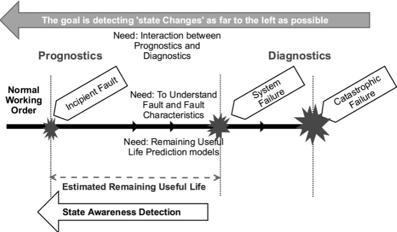
Regarding these notions, Figure 2.2 represents a typical initial fault

(46)

[image:46.595.129.524.125.356.2]

Figure 2.2: Failure progression timeline (adapted from Hess et al. (2005))

explains the role of prognostics and how the connection between prognostics

and diagnostics can be achieved. At the beginning of a system’s lifetime, all

components are in proper working order and maintenance is not necessary.

Each operational trajectory has its own specific initial health level, which is

generally stable during the early stages of use. This continues until a critical

period where an early incipient fault condition occurs. As time progresses and

operation continues, the risk of system failure, which can cause a system

dam-age and eventually a catastrophic failure, grows with time. Note that system

failure and catastrophic failure are two different points in time. The initial

de-tection of these failures and damage is always crucial to the estimation of RUL.

The detection of state changes and fault characteristics requires interactions

between prognostics and diagnostics. The goal in the timeline is improving

state awareness detection as close as possible to the point of the first incipient

(47)

In Figure 2.3 (Lewis, 2017; Goode et al., 2000), the system health

con-tinues to decrease due to the degradation process from an initial problem in

the system, and eventually reaches a critical state that causes functional

fail-ure. The system starts with a certain level of initial health and manufacturing

variation that can be considered normal, i.e., it is not representative of a fault

condition.

System Installation

Initial Problem

Stable Zone

System Health

Time

Potential Failure

Functional Failure

F P

Failure Zone

PF Interval

[image:47.595.155.487.242.508.2]

IP

Figure 2.3: System life model (adapted from (Lewis, 2017; Goode et al., 2000))

The potential failure point defines the transition from stable zone to

functional failure point. Stable zone is the time from initial machine

instal-lation to the potential failure point. This interval contains largely

condition-monitoring measurements which are randomly varying around the higher

sys-tem health limit. When the health index derived from condition monitoring

readings exceed the alarm limit of potential failure, it is assumed that the

sys-tem has entered the failure zone and will deteriorate, at an exponential rate,

(48)

zones and failure points, prognostics relate to the task of making multi-step

ahead life prediction.

The prognostic prediction is practised between the initial detection of

the failure and the progression to actual failure conditions (Lee et al., 2014).

Since the lifetime estimation is applied within the CBM domain, it includes

similar stages regarding data acquisition, signal processing and diagnostics.

For example, a typical prognostic application is a sequential process with the

following major stages in which the applications of various other CBM

appli-cations can be found (Tobon-Mejia et al., 2010; ISO-13381, 2015).

• Pre-processingdescribes any type of processing performed on raw data and pre-evaluation of existing failure modes. This step identifies the

symptom relations regarding the performance and determines the

po-tential impending failure modes.

• Existing failure mode is a step-by-step approach to identifying all existing failures in the processed data.

• Future failure mode estimates the most likely future modes, and their influence factors. Additionally, the estimated time to failure is calculated

in this mode.

• Post-action prognostics proposes the maintenance actions that need to be done. To avoid the effects of undesired failure modes, the

post-action prognostics are applied with consideration to the recommended

actions.

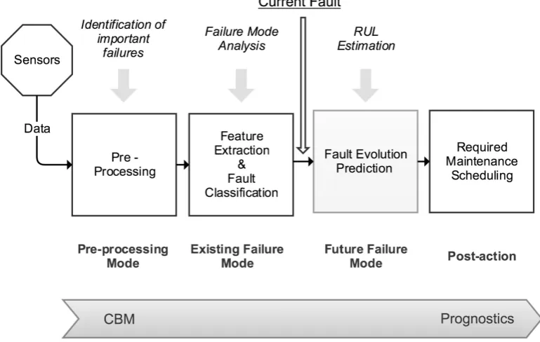
Figure 2.4 demonstrates the above-mentioned basic stages of prognosis.

The pre-processing phase receives the machinery information from sensors and

identifies important failure features that are useful for determination of any

(49)

applied for feature extraction and fault classification. Considering the current

fault level in the system, multi-step prediction is performed to calculate the

fault evolution in the future failure mode. After receiving an estimated

time-to-failure, the maintenance scheduling is performed to keep the prognostic

[image:49.595.127.512.234.478.2]

application as reliable as possible.

Figure 2.4: A Typical Prognostic Application (adapted from (Vachtsevanos et al.))

2.2.1 Prognostic Definitions

Common terms used in prognostic practice and their definitions have been

reported in several studies (Wang et al., 2004; Muller et al., 2008; Lebold and

Thurston, 2001; Byington et al., 2002). Apart from the terminology

differ-ences, these definitions mostly agree regarding the prediction aspect and RUL

estimation of the system failure (Tobon-Mejia et al., 2012). Some of these

An adaptive data filtering model for remaining useful life estimation

warwick.ac.uk/lib-publications

An Adaptive Data Filtering Model for

Remaining Useful Life Estimation

Oguz BEKTAS

Thesis

Doctor of Philosophy

Warwick Manufacturing Group

Contents

List of Tables

List of Figures

Acknowledgments

Declarations

Abstract

Symbols

Abbreviations

Chapter 1

Introduction

1.1

Motivation

1.2

Problem Statement

1.3

Research Question and Hypotheses

Research Question

Research Aim

Research Objectives

1.4

Significance and Contribution

1.5

Thesis Organisation

Chapter 2

Background and Literature

Survey

2.1

Condition Based Maintenance

2.1.1

Data Acquisition

2.1.2

Data Processing

2.1.3

Decision Making

2.2

Prognostics and Definitions

2.2.1

Prognostic Definitions