warwick.ac.uk/lib-publications
Original citation:
Allafi, Walid, Zhang, Cheng, Uddin, Kotub, Worwood, Daniel, Dinh, Quang Truong, Ascencio,
Pedro, Li, Kang and Marco, James (2018) A lumped thermal model of lithium-ion battery
cells considering radiative heat transfer. Applied Thermal Engineering, 143 . pp. 472-481.
doi:10.1016/j.applthermaleng.2018.07.105
Permanent WRAP URL:
http://wrap.warwick.ac.uk/106390
Copyright and reuse:
The Warwick Research Archive Portal (WRAP) makes this work by researchers of the
University of Warwick available open access under the following conditions. Copyright ©
and all moral rights to the version of the paper presented here belong to the individual
author(s) and/or other copyright owners. To the extent reasonable and practicable the
material made available in WRAP has been checked for eligibility before being made
available.
Copies of full items can be used for personal research or study, educational, or not-for-profit
purposes without prior permission or charge. Provided that the authors, title and full
bibliographic details are credited, a hyperlink and/or URL is given for the original metadata
page and the content is not changed in any way.
Publisher’s statement:
© 2018, Elsevier. Licensed under the Creative Commons
Attribution-NonCommercial-NoDerivatives 4.0 International
http://creativecommons.org/licenses/by-nc-nd/4.0/
A note on versions:
The version presented here may differ from the published version or, version of record, if
you wish to cite this item you are advised to consult the publisher’s version. Please see the
‘permanent WRAP url’ above for details on accessing the published version and note that
access may require a subscription.
1
A Lumped Thermal Model of Lithium-Ion Battery Cells
Considering Radiative Heat Transfer
Walid Allafi1,*, Cheng Zhang1, Kotub Uddin2, Daniel Worwood1, Truong Quang Dinh1, Pedro Ascencio Ormeno1, Kang Li3, James Marco1
1 WMG, University of Warwick, Coventry, CV4 7AL, UK
2 OVO Energy, U140-142 Kensington Church Street, London W8 4BN, UK
3 School of Electronics Electrical Engineering and Computer Science, Queen’s University Belfast
* Corresponding Author: [email protected]
Abstract:
Thermal management plays a critical role in battery operations to improve safety and prolong battery life, especially in high power applications such as electric vehicles. A lumped parameter (LP) battery thermal model (BTM) is usually preferred for real-time thermal management due to its simple structure and ease of implementation. Considering the time-varying model parameters (e.g., the varying convective heat dissipation coefficient under different cooling conditions), an online parameter estimation scheme is needed to improve modelling accuracy. In this paper, a new formulation of adaptive LP BTM is proposed. Unlike the conventional LP BTMs that only consider convection heat transfer, the radiative heat transfer is also considered in the proposed model to better approximate the physical heat dissipation process, which leads to an improved modelling accuracy. On the other hand, the radiative heat transfer introduces nonlinearity to the BTM and poses challenge to online parameter estimation. To tackle this problem, the simplified refined instrumental variable approach is proposed for real-time parameter estimation by reformulating the nonlinear model equations into a linear-in-the-parameter manner. Finally, test data are collected using a Li ion battery. The experimental results have verified the accuracy of the proposed BTM and the effectiveness of the proposed online parameter estimation algorithm.
Keywords: Lumped Thermal Model, Radiative, Nonlinear Parameter Estimation, Online Estimation Nomenclature List
BMS Battery Management System BTM Battery Thermal Model
CRTM Convection & Radiation Base Thermal Model CTM Convection Based Thermal Model
EV Electric Vehicle
ECM Equivalent Circuit Model LS Least Square
LFP LifePO4
LIB Lithium Ion Batteries
LECTM Lumped Equivalent Circuit Based Thermal Model LP Lumped Parameter
MSE Mean Square Error OCV Open Circuit Voltage RLS Recursive Least Square
SRIVC Simplified Refined Instrumental Variable Method for Continuous-Time Models
SoC State of Charge List of Symbols
Bulk Cell Density 3
[kg m ]
p
C Bulk Specific Heat Capacity 1 1
[k J kg K ]
( )
2
c
Q Convective Heat Transfer[W]
h Convective Transfer Coefficient -2 -1
W m [ K ]
e
Q Electrolyte Phase Potential[V]
r
Emissivity Coefficient
loss
Q Exchanged Heat Rate [W]
gen
Q Heat Generation Rate [W]
( )
m
T t Measured Cell Temperature[ C]o
OCV Open Circuit Voltage [V]
r
Q Radiative Heat Transfer[W]
r
h Radiative Transfer Coefficient -2 -4
W m [ K ]
s
Q Solid Phase Potential [V]
Stefan –Boltzmann ConstantA Thermal Area [M2]
List of Subscript
amb Refers to Ambient Temperature
c Refers to Convection
loss Refers to Dissipation
F Refers to Filtered Signal By 1/A
l Refers to Iteration Number
On Refers to Online Estimation
r Refers to Radiation
1
Introduction
Lithium ion batteries (LIBs) are the technology of choice in applications ranging from consumer electronic devices to electric vehicles (EVs) due to their relatively high energy and power densities. The most significant shortcoming of LIBs, however, is the changing performance and efficiency under different operation conditions [1]. Knowing and understanding varying battery properties are crucial in defining the operational capability of the battery. One of the significant factors impacting battery performance and safety is temperature [2, 3] and therefore, observing and tracking the battery temperature is one of the key functions of the battery management system (BMS) [4]. Model-based methods are typically employed for battery temperature prediction and control.
selected-3
order rational transfer function. The challenge when using reduced-order models is that although the computational time is relatively less than the time required by the electrochemical model, it is still not sufficiently efficient for online control applications [18, 19].
Another type of grey-box models is lumped-parameter (LP) model, which can be considered to be the most efficient approach in real-time thermal management applications [7, 8] due to the simplicity of parametrization and ease of implementation. The model structure is derived based on physical knowledge, while the model parameters are estimated using test data. Different types of LP BTMs have been proposed in the literature [8, 9] [20-22] [6]. For example, [20-22] [6] proposed a lumped equivalent circuit-based thermal model (LECTM) for batteries. The model can be used not only for capturing the evolution of the surface temperature, but also for the battery internal temperature prediction and estimation. The LECTM is suitable for on-board thermal management applications due to the simple model structure, low computational complexity, ease of parametrization, and acceptable accuracy. One limitation of the LECTM is that only the convective heat dissipation is considered in the heat transfer sub-model, while the heat radiation is normally neglected. The convective transfer is governed by the ambient temperature surrounding the battery while the radiative transfer is governed by the surface geometry and depends on the material, colour, and texture of the surface. In reality, this heat radiation can account for a large percentage in the overall battery heat dissipation when the ambient temperature is close to the cell temperature [6, 7, 23-25]. The contribution of the radiative heat transfer can be significant and even becomes dominant with respect to convective heat transfer as the operating temperature becomes higher [26]. A study on heat dissipation [27] showed that radiative heat from cells can constitute up to 50% of total heat dissipation during oven exposure testing. Therefore, the radiative heat transfer needs to be considered in the LECTM to better approximate the physical heat dissipation process and to improve the model accuracy. Furthermore, by including the radiative heat transfer in the BTM, the estimated convective term better represents the actual physical phenomenon, as will be explained by the experimental results in the later section.
Another key issue in the LECTM is that the model parameters depend on the environment temperature which is influenced by the ambient temperature or the flow rate of the cooling liquid. From a control aspect, the thermal management is requested, on one hand, to drive the battery within the optimal working temperature range and, on the other, to maximise the energy saving through thermal control by minimising the forced convection so that the use of the natural convection is maximised [28]. In the case of forced convection, the convective coefficient varies with the coolant mass and flow rate and is a key factor for designing the cooling system. Therefore, an online parameter estimation scheme is needed to track varying parameters of the battery model in order to improve the model accuracy for control applications.
Once the model structure is determined, the next step is to estimate the parameters. The simplified refined instrumental variable method in continuous-time domain (SRIVC) has been employed to estimate the parameters [29]. The SRIVC is the direct parameter estimation approach employing a filter and instrumental variables (IVs) to provide an optimal statistical solution of parameter estimation for the selected thermal model with noises. To deal with the problem of time-varying model parameters of the LECTM, The adaptive SRIVC method is adopted, which can, in iterative manner, optimise the filter parameters and generates estimates that are asymptotically efficient (minimum variance) and consistent. The resulted optimal filter is therefore more adaptable compared to the user-defined ones in the traditional approaches, such as the state variable filter or generalised Poisson moment functional methods. Moreover, the SRIVC method offers a rapid convergence, providing consistent and asymptotically unbiased parameter estimates even facing with non-uniform white noises [30, 31].
4
This paper is organised as follows, Sections 2 addresses the thermal model derivation from first principle while Section 3 shows the reformulation for descripting the model in a linear-in-the-parameter way. The simplified refined instrumental variable methods for off-line and online parameter estimation are addressed in Section 4 and 5, respectively. The experimental data is presented in Section 6 and this data is used for model parameter estimation using the method given in Sections 3 and 4. The results of off-line model comparison and online parameter estimation are discussed in Section 7. Finally, conclusions and further work are presented in Section 8.
2
Lumped Parameter Simplified Heat Transfer Model Description
Conservation of energy for a Li-ion cell with lumped thermal capacity balances accumulation, heat dissipation, and heat generation terms as:
gen loss
( )
( ) ( )
dT t
c Q t Q t
dt (1)
which describes the evolution of cell temperature T, with time. In (1),cCp is the battery thermal capacity,
whereis the bulk cell density 3
[kg m ] , Cp the bulk specific heat capacity 1 1
[k J kg K ] , Qgen( )t is the heat
generation rate in the battery [W] and Qloss( )t the heat exchanged with the surrounding environment, which is given by the sum of the convective and radiative heat transfer terms. The convective heat transfer term is expressed through Newton’s law as:
amb
( ) ( ) ( )
c c
Q t h T t T t (2)
where Tamb( )t is the ambient temperature and hc hA , where h is the convective transfer coefficient -2 -1
W m
[ K ] and A the thermal area [m2]. The radiative heat transfer follows the Stefan-Boltzmann law, expressed as follows:
4 4
( ) ( ) ( )
r r amb
Q t h T t T t (3)
where hr A, where
is the emissivity coefficient which defines how efficiently the surface emits energy relative to a blackbody and
the Stefan –Boltzmann constant(5.67 10 [W m 8 -2K-4]).There are four sources of heat generation in a lithium ion battery under charging/discharging operations, including: heat generated from resistive dissipation (Joule heating), the entropy of the cell reaction, side reactions and the heat of mixing [32]. As shown by Uddin et al. [33], in operation, Joule heating dominates heat generation. Physically, this contribution to heat generation represents the irreversible resistive dissipation caused by the deviation of the surface over-potential, which is the difference between the solid phase potential Q ts( ) and
electrolyte phase potential Q te( ), from the volume averaged open circuit voltage (OCV) due to a resistance of the
passage of current (𝑖) and is expressed as:
( ) ( ) ( ) ( )
gen
Q t i t v t OCV t (4)
where ( )i t and ( )v t are the measurable current and terminal voltage respectively. OCV t( ) is the battery OCV
that can be obtained from Galvanostatic Intermittent Titration Tests [34] and is a function of state of charge (SoC). It is assumed that the battery SOC (and thus OCV) is obtained through coulomb counting or other existing techniques such as those presented in [1, 35, 36].
This paper considers two scenarios for heat dissipation, Qloss( )t . The first model only considers the convective
5
3
Problem Reformulation
The CRTM is the nonlinear model with respect to cell temperature, due to the fourth order temperature terms arising from the radiative heat transfer defined in (3). This may lead to problems with commutitive properties of the filter with the nonlinear ordinary differential equations, see [37]. To deal with this problem, the CRTM is reformulated to be a linear-in-the-parameters model. Hence, the CRTM in (1) can be described by the multi-input single-output ordinary differential equation, expressed in a polynomial form as:
4 4 0 ( ) ( ) ( ) ( ) ( ) ( ) ( ) ( ) ( ) ( ) ( ) gen r ambg gen r r amb
m
Q t i v t OCV t
K t T t T
A T t b Q t b K a T
T t T t e t
(5)
where T tm( ) is the measured temperature, ( )e t represents the measuring noise which is assumed to be white (zero
mean) noise, the ambient temperature Tamb is assumed constant and the nonlinear term 4
( )
T t can be
approximated as 4 4
( ) m( )
T t T t [37] (because the signal to noise ratio is large in the case of the T tm( )).A
is the output polynomial obtained from (1) and (2), and expressed as:
0A a (6)
where a0 hc c
, bg 1 c
, r r
h b
c
and the differential operator is defined such that d
dt
. It can be noted
that the derivative term of the ambient temperature ( Tamb) is neglected because the ambient temperature is
assumed to be constant.
The CTM is a special case of the CRTM whenbr Kr 0. This leads to the removal of all the radiative terms in (5).
4
SRIVC Method for Thermal Model
In this section, the SRIVC method is adopted for the model parameter estimation. The minimised error function is given by:
0
( ) ( ) ( ) ( )
( ) ( ) ( )
g r
T m gen r amb
b b a
t T t Q t K t T
A A A
(7)where the ambient temperature Tamb is assumed to be constant. Considering zero initial conditions, the Laplace
transform of (7) is given as:
0( ) ( ) g ( ) r ( ) ( )
T m gen r amb
b b a
s T s Q s K s T s
A s A s A s
(8)
where Tamb
s 1Tamb s and the Laplace transform of the output polynomial is expressed as:
0A s s a (9)
To approximate the derivative terms, while retaining T( )s on the left-hand side of (8) without filtering, a filter
1
A s is introduced in the first term on the right-hand side of (8). This leads to the introduction of an output
6
0
1 1 1 1
( ) ( ) ( ) ( ) ( )
T s A s T sm bg Qgen s br K sr a Tamb s
A s A s A s A s
(10)Equation (10) can then be transformed back to the time-domain as:
0
1 1 1 1
( ) ( ) ( ) ( ) ( )
( ) ( ) ( ) ( )
T t A T tm bg Qgen t br K tr a Tamb
A A A A
(11)Equation (11) can be expressed in the filtered form as:
, , , 0 ,
( )t A( )Tm F( )t bg( )Qgen F( )t br( )Kr F( )t a Tamb F( )t
(12)
where , , , , 1 ( ) ( ) ( ) 1 ( ) ( ) ( ) 1 ( ) ( ) ( ) 1 ( ) ( )
m F m
gen F gen
r F r
amb F amb
T t T t
A
Q t Q t
A
K t K t
A
T t T
A (13)
Subsequently, the expression (12) is re-arranged into a pseudo-regression form, which can be solved using the least squares (LS) solution:
, ( ) ( ) ( )
T
m F tk F tk tk
T (14)
where the index ‘k’ indicates the sample number and thusTm F, ( )tk is the sampled form of Tm F, ( )t , the ( ) tk is
the modelling error, and T F
and are in turn the regression and parameter vectors given as:
, , , ( ) ,
( ) ( ) ( ) ( ) T
T
F tk Tamb F tk Tm F tk QgenF tk KrF tk
(15)0 g r
a b b
7
The block diagram of the filter in (13) which can be mapped into Simulink is given in Figure 1. Figure 1 shows how the filter can generate the Tm F, ( )tk signal and their derivatives fromT tm( )k .
The SRIVC method is implemented as a two-stage algorithm provided below:
Stage 1: The initial model parameters of the output polynomial need to be obtained for the purpose of deducing the time derivatives of the output signals, which are subsequently used in stage 2. Several existing techniques such as state variable filtering can be applied for this purpose. The obtained initial parameters are used by the stable filter, whose the denominator has the same order as the output polynomial ( )A , i.e.,
1 1
F
(17)
The parameters in (16) can be initialised as
b
ˆ ( ) 1
g
0
,bˆ ( ) 0r 0 , and aˆ ( ) 10 0 , where hatted symbols represent the estimated values.Stage 2: Iteratively repeat steps (I) to (IV), defined below, until the sum of the square difference between ˆl and
1 ˆ
l
is satisfactorily small, for example
25 1
ˆ ˆ 10
l l
where the subscript l indicates the current iteration step and l1 indicates the previous iteration step.I. Generate the simulated output to be instrumental variable:
1 1 1
1 1
0
1
ˆ ( ) ˆ( ) ˆ ( )
ˆ( ) ˆ ( ) ˆ ( ) ˆ
( , ) ( , ) ( , )
l l l
l l l
g r
gen r amb
b b a
T t Q t K t T
A A A
(18)
II. Pre-filterTm, Tˆ, Qgen, Kr and Tambusing ˆ( , )A i in (13) and Figure 1.
III. Extract the parameters using an instrumental variable LS procedure:
1
.
1 1
1 N ˆ 1 N ˆ
T
F k F k F k m
i F k
k k
t t t T t
N N
(19)
0
a
Interpolator
T
m F,
t
T
m F,
t
T
m F,
t
k
, m F k
T
t
, m FT
t
m k [image:8.595.75.516.77.281.2]T t
T t
m
8 where the regression vector T
F
is obtained by (15) and the regression vector of instrumental variables,
ˆF tk
, is defined as follows:
. ˆ ( ) , ( ) ˆ , ()ˆF tk Tamb F TF tk Qgen F t Kr F t
(20)IV. Update
b
ˆ ( )
g
l , ˆ ( )br l , ˆ( , )A l and aˆ ( )0 l .The above procedure identifies offline the model parameters, which will further be used as initialization of the online parameter estimation procedure in the next section.
5
Online Parameter Estimation and Updating
This section presents how the convective coefficient can be online tracked, as this convective coefficient depends on the heat dissipation condition, i.e., natural or forced air convection. On the other hand, both the thermal capacitance and the radiative coefficient are assumed to be constant [38] and obtained from off-line model estimation using the experimental data.
The regression vector in (14) is reformulated and expressed as:
,
( ) T ( ) ( )
k On F k On k
y t t t (21)
where the subscript On refers to online and On a0, T , ( ) , , ( )
On F tk Tamb F TmF tk
and the output ( )y tk is calculated using heat generations and the estimated radiative heat transfer as:
,
ˆ
,( )
ˆ
,( )( )
( )
kT
m F( )
kb Q
g gen Ft
kb K
r r Ft
ky t
t
t
(22)Following the classical derivation of the recursive LS (RLS) algorithm with an inherent mechanism for tracking time-varying parameters, the general form of the RLS is expressed as [31]:
, 1 , , , 1 , 1( ) 1 ( ) ( )
ˆ ( ) ˆ ( ) ( ˆ
ˆ ˆ
ˆ
) ( )
1
( )
k k On F k On F k k On F k
On k On k k k k On k
k k k On F k k
T
T On F
T
L t P t t t P t t
t t L t y t t t
P t P t L t t P t
(23)
where P is the parameter covariance matrix. The initial values of (0)P are selected as (0)P I where
0and I is an identity matrix while is the forgetting factor. In this paper, these parameters are selected such as
0.9999
to avoid parameter fluctuation [31] and 4
(0) 10
P I. This is because On(0)is the estimated
vector, ,
,1
0ˆ ˆ 0
k
On l k On
t t
, derived from the off-line SRIVC estimation (l represents the iteration number
and l1 in the case of the initial value). This means there is no need for large corrections.
The iterative online estimation process at each time tk is summarised as follows:
I. Set l1,
ˆ
On,1
t
k
ˆ
On
t
k1 . II. Update Aˆ
,
ˆOn l,1( )tk
in (13).III. Filter Tm, Qgen, Kr and Tambusing Aˆ
,
ˆOn l,1( )tk
as given in (13).9
VI. Steps II to V are repeated for fouriterations where convergence of the parameter is very rapid. It requires two or three iterations, for convergence analysis, see [39].
VII. Set
ˆ
On
t
k
ˆ
On,4
t
k .6
Experimental Setup
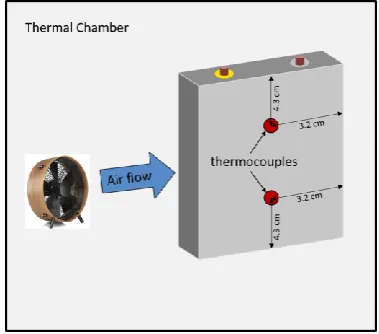
In this work, commercially available Li-ion prismatic cells with a LiFePO4 (LFP) cathode and LiC6 (graphite) anode were used. An electronic charger and an electronic load were used to cycle the battery. The test procedure was controlled by a NI Compact-RIO system, which also logged the test data, including the voltage, current and temperature measurements. The rated capacity and nominal voltage of the cells are 10 Ah and 3.2V, respectively. The battery casing is made of Aluminium with dimensions 13.0 x 6.8 x 1.8 cm. Two thermocouples were attached to the battery shell surface, as illustrated in Figure 2. In order to isolate the effect of fluctuating ambient temperatures, all the tests were carried out at 25℃ within an environmental chamber. The battery was cycled using a programmable charger and an electronic load (with associated monitoring and control software) to generate the DC load profile. The difference between the two temperature measurements was within 2 ℃ and therefore, either one could be selected as the approximate overall cell temperature. The maximum current rate is 3C, i.e., 30A, and the limit voltage for charging and discharging are 3.65V and 2.5V, respectively.
The experiments were conducted at the EV and Smart Grid Lab, Queen’s University Belfast and experimental data under two different heat dissipation scenarios were collected for comparison. Each test dataset consisted of a sequence of charging/discharging at different rates, and two self-heat tests using 3C pulsed charging-discharging were also applied to raise the cell temperature to a higher level. The sampling interval is 0.5 [s] for the current, voltage and temperature measurements.
[image:10.595.202.392.471.638.2]The test data are collected under two different heat dissipation conditions. Datasets 1 and 2, illustrated in Figure 3, were collected under natural air convection. One data set was used for modelling training processes and the other one was used for validation. While forced air convection using a fan was employed when collecting test data set 3, as shown in Figure 4. Due to the different heat dissipation conditions, the thermal model parameters will be different. This data set was then used for investigating the online parameter estimation scheme presented in Section 5.
11
Figure 3: Two natural convection data sets, one for modelling and the other for validation, are presented in black solid and grey solid lines, respectively where (A) shows current profile, (B) shows measured voltage (C) gives approximated SoC using coulomb counting approach given in [36] and (D) shows heat generation profile corresponding to (4) and self-heat test
12
Figure 4: Forced convection data is presented in (A) the current profile, (B) the measured voltage (C) the approximated SoC and (D) the heat generation profile corresponding to (4) and self-heat test part is from 7.8-8.4 [hr] in (A, B and D) and
13
7
Results and Discussion
The model evaluation process can be divided into different phases as summarised below:
i. Experimental phase: this phase is to collect a set of data including the battery current, voltage and
temperature for natural and forcing convection scenarios (Section 6)
ii. Offline modelling and validation: the collected data under the natural convection (datasets 1 and 2)
is used for the offline parameter estimation of CTM and CRTM and model validation, using the
algorithm in Section 4.
iii. Online modelling: The test data under the forced convection (dataset 3) is used for validating the
online parameter estimation scheme. Here, the offline estimated CRTM parameters are used as
parameter initialization for the online estimation.
iv. The results obtained from ii and iii are then discussed.
7.1 Offline model parameter estimation results
This section presents a comparison of the modelling accuracy between the CTM and CRTM. The parameters of CTM and CRTM have been estimated offline using the first dataset under the natural air convection as shown in Figure 3 by the SRIVC method presented in Section 4. The resulted parameters of both models are given as follows,
CTM ˆ 399.7922 13 21 ˆ .01 c h CRTM 10 ˆ ˆ ˆ 418.1638 8.0887 9.9136 10 r c h h
The total exposed battery surface area is A0.0248 m2. Therefore, the estimated radiative coefficient (
10 -4
10
9.9136 W.K ) gives rise to the battery surface emissivity, an amount of 10 8 10 0.024 9.913 8 6 0.70 5.67 10 5
r h A
, which is in line with the range of reported emissivity values for the surface of lithium ion batteries [27]. Another critical result is the convective coefficient ˆh. According to physical
analysis [38, 40, 41], typical values for natural convection coefficients with air lie between 1 10 W.m .k -2 1.
Therefore, compared to the traditional CTM, the CRTM gives rise to the modelling accuracy in term of representing the physical thermal convective process. To sum up, the estimated parameters of the CRTM model are more in accordance with the physical interpretation, which can be therefore effectively support the online thermal estimation using the proposed approach.
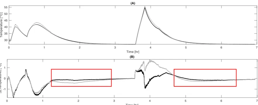
The training results of both the models are then plotted in Figure 5. The results show the good performance of both models. The peak errors were observed during the fast temperature changes, which was probably caused by the model order reduction from the physical process. However, the modelling errors of the CTM and CRTM were in turn less than 1.2 and 1 C0 , which were acceptable for battery applications.
In terms of the modelling accuracy, the CRTM showed the better performance compared to that of the CTM, as analysed in Figure 5 (B). The mean square error (MSE) generated by the CTM was 0 2
14
than three times lower for the CRTM, 0.0724 C . This was expected since the latter was the higher fidelity 0 2
model accounting for the radiation factor.
Next, the models with the trained parameter sets were validated using the second data set (Figure 3). The similar performance were then obtained as shown in Figure 6. The corresponding MSEs were 0 2
0.3434 C and 0 2
0.1889 C
for the CTM and CRTM, respectively.
[image:15.595.77.520.242.410.2]It also can be observed from Figure 5 and 6 (as indicated by the ‘red’ boxes) that the CRTM could fit the heat dissipation nonlinearity during the temperature relaxation process more accurately than the CTM model. This implies the effectiveness of considering the radiative heat generation in designing the thermal model.
Figure 5: Modelling performance of CTM and CRTM for temperature prediction where (A) shows the actual temperature, predicted temperature using CTM and predicted temperature using CRTM, presented in dotted-black line, solid grey and solid black lines, respectively; and (B) presents the difference between the actual and predicted temperature using CTM in
grey solid line and using CRTM in black solid line.
[image:15.595.81.522.514.694.2]15
16 7.2 Online estimation of the convective coefficient
The test dataset 3 under forced air convection is used here to validate the adaptive parameter estimation scheme presented in Section 6. The CRTM model parameters offline estimated using dataset 1 under natural convection,
(cˆ 418.1638, hˆ 8.0887, hˆr 9.9136 1010
as presented in Section 7.1), were used to initialise the parameter
estimation. The heat conductivity under forced air convection ˆh will become higher compared with natural convection. The online estimation scheme for the convective coefficient was integrated such that the evolution of
c h h
A
of the thermal model in (2) can be well forecasted in order to improve the accuracy of the thermal
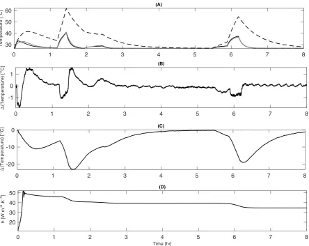
prediction. The goal is to achieve a smooth parameter convergence with a small error rather than fast convergence with a lot of fluctuations. The battery temperature prediction was carried out using both the CTM and CRTM models and the results were plotted in Figure 7 (A).
As seen in this figure, the prediction performance using the CTM was very poor with more than 20oC modelling error (black dashed line in Figure 7 (A)). The main reason was the CTM model with its fixed parameters was derived from the different cooling condition. Hence to improve the thermal prediction accuracy, it is necessary to update the model parameters online to adapt to the condition changes. This could be well addressed using the developed online parameter estimation approach.
For the CRTM model, the convective coefficient was online one-step-ahead regulated based on the prediction error. As the result, the prediction performance was significantly improved compared to that of the constant-parameter CTM. The maximum prediction error in this case was only around 1.5oC. Figure 7 (C) shows how the convective coefficient behaved under the forced cooling scenario. The initial value of the convection coefficient,
2 -10
8.09 [
m K ]
ˆ
/
W
c
h
t
h
A
, was derived under the nature convection condition. It can be seen from Figure 7 (D) that there was a large convergence of ˆ( )h t toward -2 -452 [W m K ]in the first 10 minutes which then
settled to 2 -1
[W m K ] ˆ( ) 48
h t . The increase in the convective coefficient is due to the increase in the air fluid velocity and this matches the forced convictive description given in [42]. The peak value of ˆh was at t 0.2 [hr] and the rapid convergence was due to the large error at the initiation shown in Figure 7 (B), which represents the transient stage. When the modelling error occurs as shown in Figure 7 (B), there is a corresponding correction of the model parameter from RLS as illustrated in Figure 7 (D). This can be noted at around
0.15 [hr], 1.3 [hr], 2.3 [hr], 5.8 [hr]
17
Figure 7: The results of online estimation of the convective coefficient and temperature prediction of thermal model using test data set 3, shown in Figure 4 where (A) shows the actual temperature profile in black solid line, predictive using the offline model in black dashed line and predicted using online model with using the online estimated convection coefficient presented in (D); (B) gives the error between the actual and online estimated temperature; (C) presents the error between the
18 7.3 Radiation and convection heat transfer analysis
To show the necessity of including the radiative term in the thermal model, the quantities of the radiation and convection heat transfer were compared. Figure 8 (A,B) show that the radiative heat transfer was relatively significant compared with the convective heat transfer in case of the natural convection. Values for the estimated radiative coefficient ( 10 -4
10
9.9136 W.K ) give rise to a calculated battery surface emissivity value of 0.702 which is in line with the range of reported emissivity values for the surface of lithium ion batteries [27]. Under forced air convection, the conductivity coefficient increased noticeably, leading to a reduced portion of the radiation transfer in the overall heat dissipation, as shown in Figure 8 (C).
The rise in the estimated convective coefficient, shown in Figure 7 (C) in the first half an hour, causes a large decrease in the importance of the radiative heat transfer relative to the forced convection. Nevertheless, as the estimated convective coefficient converged to approximately 0.9 during the remaining simulation time, as shown in Figure 8 (C) the radiative heat transfer term becomes more significant.
[image:19.595.98.491.343.623.2]Therefore, this proposed model can be significant for prediction and monitoring applications in the case of natural convection, low forced convection or natural-forced convection, where the radiative heat dissipation plays a significant part. Furthermore, the online estimation of the convective coefficient offers a better modelling performance for the control and management applications when it is not always under a constant forced convection.
Figure 8: Estimated convection and radiation heat transfer, given in (2) and (3), are presented in black-sold and grey-slid lines, respectively, where (A) shows the estimated convection and radiation heat transfer with natural convection for modelling data, (B) shows the estimated convection and radiation heat transfer with natural convection for validation data and (C) presents the estimated convection and radiation heat transfer of the online estimation.
19
8
Conclusions and further work
8.1 Conclusions
In this paper, a novel algorithm is proposed that directly estimates the model parameters of a nonlinear lumped BTM from observed cell-level data. The parameter estimation algorithm extends the simplified refined instrumental variable method to estimate the parameters by reformulating the original equations to be described as a multi-input/single-output linear model. The recursive form SRIVC is used for online parameter estimation of the proposed model. The online estimation is used to track the variation of the convective coefficient due to forced convection, leading to more accurate temperature estimations.
The suitability of the models presented in this paper is application and environment dependent. The proposed radiation coupled model is shown to be more accurate in the case of natural convection, low forced convection or natural-forced convection. The online estimation of the convective coefficient offers a better performance for the control and management applications when it is not always under a constant convection.
8.2 Further work
The models developed did not consider the non-uniform temperature distribution and the conduction heat transfer inside the battery. Further work thus will focus on improving the proposed model to take these factors into consideration by simplification of the classical thermal governing equations. There is a potential to use the fractional order transfer function to approximate the transcedual transfer function of the thermal system by assuming the conductive coefficient to be constant.
9
List of References
[1] W. Allafi, K. Uddin, C. Zhang, R. Mazuir Raja Ahsan Sha, J. Marco, On-line scheme for parameter
estimation of nonlinear lithium ion battery equivalent circuit models using the simplified refined
instrumental variable method for a modified Wiener continuous-time model, Applied Energy, 204
(2017) 497-508.
[2] K. Uddin, S. Perera, D.W. Widanage, L. Somerville, J. Marco, Characterising Lithium-Ion Battery
Degradation through the Identification and Tracking of Electrochemical Battery Model Parameters,
Batteries, 2 (2016).
[3] D.H. Doughty, E.P. Roth, A general discussion of Li ion battery safety, The Electrochemical Society
Interface, 21 (2012) 37-44.
[4] M.A. Hannan, M.S.H. Lipu, A. Hussain, A. Mohamed, A review of lithium-ion battery state of charge
estimation and management system in electric vehicle applications: Challenges and
recommendations, Renewable and Sustainable Energy Reviews, 78 (2017) 834-854.
[5] (!!! INVALID CITATION !!! [5, 6]).
[6] X. Lin, H.E. Perez, J.B. Siegel, A.G. Stefanopoulou, Y. Li, R.D. Anderson, Y. Ding, M.P. Castanier,
Online Parameterization of Lumped Thermal Dynamics in Cylindrical Lithium Ion Batteries for Core
Temperature Estimation and Health Monitoring, IEEE Transactions on Control Systems Technology, 21
(2013) 1745-1755.
[7] C. Zhang, K. Li, J. Deng, S. Song, Improved Realtime State-of-Charge Estimation of LiFePO4 Battery
Based on a Novel Thermoelectric Model, IEEE Transactions on Industrial Electronics, 64 (2017)
654-663.
[8] C. Zhang, K. Li, J. Deng, Real-time estimation of battery internal temperature based on a simplified
thermoelectric model, Journal of Power Sources, 302 (2016) 146-154.
[9] T.P. Bohlin, Practical grey-box process identification: theory and applications, Springer Science &
Business Media, 2006.
20
[11] M. Xu, Z. Zhang, X. Wang, L. Jia, L. Yang, A pseudo three-dimensional electrochemical–thermal
model of a prismatic LiFePO4 battery during discharge process, Energy, 80 (2015) 303-317.
[12] C.Y. Wang, V. Srinivasan, Computational battery dynamics (CBD)—electrochemical/thermal
coupled modeling and multi-scale modeling, Journal of Power Sources, 110 (2002) 364-376.
[13] F. Bahiraei, M. Ghalkhani, A. Fartaj, G.-A. Nazri, A pseudo 3D electrochemical-thermal modeling
and analysis of a lithium-ion battery for electric vehicle thermal management applications, Applied
Thermal Engineering, 125 (2017) 904-918.
[14] S. Panchal, I. Dincer, M. Agelin-Chaab, R. Fraser, M. Fowler, Thermal modeling and validation of
temperature distributions in a prismatic lithium-ion battery at different discharge rates and varying
boundary conditions, Applied Thermal Engineering, 96 (2016) 190-199.
[15] X. Feng, L. Lu, M. Ouyang, J. Li, X. He, A 3D thermal runaway propagation model for a large format
lithium ion battery module, Energy, 115 (2016) 194-208.
[16] Q.-K. Wang, Y.-J. He, J.-N. Shen, Z.-F. Ma, G.-B. Zhong, A unified modeling framework for
lithium-ion batteries: An artificial neural network based thermal coupled equivalent circuit model approach,
Energy, 138 (2017) 118-132.
[17] B.C. Ng, I.Z.M. Darus, H. Jamaluddin, H.M. Kamar, Application of adaptive neural predictive
control for an automotive air conditioning system, Applied Thermal Engineering, 73 (2014) 1244-1254.
[18] M. Muratori, M. Canova, Y. Guezennec, G. Rizzoni, A Reduced-Order Model for the Thermal
Dynamics of Li-Ion Battery Cells, IFAC Proceedings Volumes, 43 (2010) 192-197.
[19] Z. Deng, H. Deng, L. Yang, Y. Cai, X. Zhao, Implementation of reduced-order physics-based model
and multi-parameters identification strategy for lithium-ion battery, Energy, 138 (2017) 509-519.
[20] J. Sun, G. Wei, L. Pei, R. Lu, K. Song, C. Wu, C. Zhu, Online Internal Temperature Estimation for
Lithium-Ion Batteries Based on Kalman Filter, Energies, 8 (2015) 4400.
[21] K. Smith, G.-H. Kim, E. Darcy, A. Pesaran, Thermal/electrical modeling for abuse-tolerant design
of lithium ion modules, International Journal of Energy Research, 34 (2010) 204-215.
[22] Y. Xiao, B. Fahimi, State-space based multi-nodes thermal model for Lithium-ion battery, in: 2014
IEEE Transportation Electrification Conference and Expo (ITEC), 2014, pp. 1-7.
[23] C. Forgez, D. Vinh Do, G. Friedrich, M. Morcrette, C. Delacourt, Thermal modeling of a cylindrical
LiFePO4/graphite lithium-ion battery, Journal of Power Sources, 195 (2010) 2961-2968.
[24] F. He, X. Li, L. Ma, Combined experimental and numerical study of thermal management of battery
module consisting of multiple Li-ion cells, International Journal of Heat and Mass Transfer, 72 (2014)
622-629.
[25] R.R. Richardson, P.T. Ireland, D.A. Howey, Battery internal temperature estimation by combined
impedance and surface temperature measurement, Journal of Power Sources, 265 (2014) 254-261.
[26] M. Shadman Rad, D.L. Danilov, M. Baghalha, M. Kazemeini, P.H.L. Notten, Adaptive thermal
modeling of Li-ion batteries, Electrochimica Acta, 102 (2013) 183-195.
[27] T.D. Hatchard, D.D. MacNeil, D.A. Stevens, L. Christensen, J.R. Dahn, Importance of Heat Transfer
by Radiation in Li
‐
Ion Batteries during Thermal Abuse, Electrochemical and Solid-State Letters, 3
(2000) 305-308.
[28] W. Liu, Introduction to Hybrid Vehicle System Modeling and Control, 2013, in, Wiley.
[29] G.P. Rao, H. Unbehauen, Identification of continuous-time systems, IEE Proceedings - Control
Theory and Applications, 153 (2006) 185-220.
[30] X. Liu, J. Wang, W.X. Zheng, Convergence analysis of refined instrumental variable method for
continuous-time system identification, IET Control Theory & Applications, 5 (2011) 868-877.
[31] P.C. Young, Recursive estimation and time-series analysis: An introduction for the student and
practitioner, Springer Science & Business Media, 2011.
[32] K.E. Thomas, J. Newman, Thermal modeling of porous insertion electrodes, Journal of the
Electrochemical Society, 150 (2003) A176-A192.
21

![Figure 4: Forced convection data is presented in (A) the current profile, (B) the measured voltage (C) the approximated SoC and (D) the heat generation profile corresponding to (4) and self-heat test part is from 7.8-8.4 [hr] in (A, B and D) and zoomed in](https://thumb-us.123doks.com/thumbv2/123dok_us/9427548.447372/13.595.83.502.83.656/figure-convection-presented-current-measured-approximated-generation-corresponding.webp)