Reducing Binary Quadratic Forms for More Scalable Quantum
Annealing
Georg Hahn
Imperial College, London, UK
Hristo Djidjev (PI)
Los Alamos National Laboratory
Abstract
Recent advances in the development of commercial quantum annealers such as the D-Wave 2X allow solving NP-hard optimization problems that can be expressed as quadratic uncon-strained binary programs. However, the relatively small number of available qubits (around 1000 for the D-Wave 2X quantum annealer) poses a severe limitation to the range of problems that can be solved. This paper explores the suitability of preprocessing methods for reducing the sizes of the input programs and thereby the number of qubits required for their solution on quantum computers. Such methods allow us to determine the value of certain variables that hold in either any optimal solution (called strong persistencies) or in at least one optimal solution (weak persistencies). We investigate preprocessing methods for two important NP-hard graph problems, the computation of a maximum clique and a maximum cut in a graph. We show that the identification of strong and weak persistencies for those two optimization problems is very instance-specific, but can lead to substantial reductions in the number of variables.
1
Introduction
1.1 Quantum annealing and D-Wave
The recent availability of the first commercial quantum computers of D-Wave Systems Inc. (D-Wave, 2016) provides a novel tool to help finding, by a process known asquantum annealing, global solutions to NP-hard problems that seem to be difficult to obtain classically (Djidjev et al., 2017). As of 2017, the most recent version of the company’s quantum annealer, D-Wave 2000Q, is capable of handling around 2000 qubits of quantum information. Each qubit consists of a super-conducting loop on the D-Wave chip which simultaneously encodes a quantum superposition of−1 and +1 via two superimposed currents in both clockwise and counter-clockwise directions (Johnson et al., 2011; Bunyk et al., 2014). Upon completion of the annealing process, the system turns classical and each qubit takes a classical (binary) value that can be read and assigned to a variable. D-Wave is designed to minimize an objective function consisting of a sum of linear and quadratic binary contributions, given as
H=H(x1, . . . , xN) = X
i∈V
aixi+ X
(i,j)∈E
aijxixj, (1)
where ai, aij ∈ R and V = {1, . . . , N}, E = V ×V for N ∈ N qubits (King et al., 2015). The
functional type (1) is called the Hamiltonian encoding the energy of a quantum system. In (1) qubits are encoded by variables xi, E denotes the dependency structure between the qubits (the set of interactions), and ai and aij encode physical characteristics of the qubits and the links (calledcouplers) between them, respectively. During annealing, the quantum system tries to reach
a configuration of minimal energy of H. A quadratic form of type (1) withxi ∈ {−1,1} is called an Ising model. By replacing xi in (1) with (xi + 1)/2, one gets a quadratic form of the same type as (1), but with xi ∈ {0,1}. The resulting problem is called a quadratic unconstrained binary optimization (QUBO) problem. Any QUBO or Ising problem can be solved on D-Wave as long as there are enough qubits and couplers between those qubits available on the D-Wave architecture to represent the system (1).
1.2 Aim of this work
Although Djidjev et al. (2017) show that certain instances designed to fit the D-Wave qubit inter-connection network can be solved magnitudes faster with D-Wave than with its classical analogues, the limitation of only around 1000 qubits and about 3000 couplers available on D-Wave 2X (DW) at Los Alamos National Laboratory poses a severe restriction. For most NP-hard optimization problems, due to the density of the HamiltonianH, the largest problems able to fit DW are of size about only 45.
To mitigate the current size limitations of the D-Wave architecture, this work tries to explore the usability of preprocessing methods allowing to determine the value of certain variables in a QUBO or Ising problem. Fixing all such variables then results in a new Hamiltonian of reduced size, consisting only of the unresolved variables. We investigate the usage of partitioning and roof duality methods for two important NP-hard graph problems, the Maximum Clique and the Maximum Cut problem, which have multiple applications including network analysis, bioinformatics, and computational chemistry. Given an undirected graph G= (V, E), a clique is a subset S of the vertices forming a complete subgraph, meaning that any two vertices ofS are connected by an edge inG. The clique size is the number of vertices inS, and theMaximum Clique problem is to find a clique inGwith a maximum number of vertices (Balas and Yu, 1986). A cutS of a graph Gis the set of (cut) edges betweenS and V \S inG. The Maximum Cut problem is to find a maximum cut, which is a cut of maximum size.
1.3 Previous work
In Boros and Hammer (2001), optimization methods for quadraticpseudo-boolean functions, which are multi-linear polynomial functions of boolean variables, are considered. The authors analyze a variety of techniques based on roof duality, introduced in Hammer et al. (1984), in order to deter-mine partial assignments of values or relations between variables in such pseudo-boolean functions. A comprehensive overview of efficient preprocessing techniques for QUBO optimization can be found in Boros et al. (2006): Those techniques consists of methods based on first and second order derivatives, roof duality and probing techniques resulting in lower bounds on the minimum energy of a QUBO, the values in either any (strong persistencies) or at least one optimum (weak persis-tencies), binary relations between variables in some or every optimum, as well as decomposition techniques of the original problem into several smaller pairwise independent QUBO subproblems.
A more efficient implementation of the probing techniques of Boros et al. (2006), combined with the aforementioned roof duality, is presented in Rother et al. (2007), with a special focus on computer vision applications. The code for the methods investigated in Rother et al. (2007) are made available for C++ in the Qpbo package of Kolmogorov (2014). Bindings of this package for Python are available (packagePyQpbo, which is part of thePyStruct package of M¨uller and Behnke (2014)) and will be used in the experiments of this article.
graph problems we consider, Maximum Clique and Maximum Cut, are given. Section 3 focuses on the Maximum Clique problem. We state its formulation as a QUBO, highlight the use of a decomposition method based on graph partitioning methods into smaller subproblems, and present experimental results for Qpbo. For this we employ several test graphs, both stand-alone and in connection with the decomposition approach. Section 4 repeats the QUBO formulation and a Qpbo experimental study for the Maximum Cut problem. We conclude with a discussion in Section 5.
In the rest of the paper, we denote a graph as G= (V, E), where V ={1, . . . , n} is a set of n
vertices andE is a set of undirected edges.
2
Background
We briefly overview the techniques used in Boros et al. (2006) and Rother et al. (2007) in order to identify strong and weak persistencies. Given a QUBO instance, it is first represented as a (quadratic)posiform
φ(x) = X T⊆L
aT Y
u∈T
u, (2)
where aT ≥ 0 for all T 6= ∅ and L is a set of literals over the n variables {1, . . . , n} and their complements. It is shown in Boros et al. (2006) that any posiform (2) can be equivalently expressed as a quadratic form
Φ(x) =a0+
X
u∈L
auu+ X
u,v∈L
auvuv.
Moreover, Boros et al. (2006) shows that there is a one-to-one correspondence between posiforms and implication networks, which are capacitated networks GΦ = (V, E) with n = |V| nodes and
non-negative capacitiesγuvon the edges connecting any two nodesu, v∈V,u6=v,V ={1, . . . , n}. The implication network GΦ has an important application in the computation of theroof dual,
which is a lower bound on the value of a quadratic posiform (Hammer et al., 1984). The roof dual is computed with the help of a maximum flow through the implication networkGΦ.
More importantly for our work, the flow analysis of the implication network also identifies strong and weak persistencies for problem (2), which are then transformed for persistencies for problem (1).
As shown in Boros et al. (2006), the effectiveness of the roof duality method for finding persis-tencies can be improved by usingprobing, which is a method that assigns values of 0 and 1 to some variables and then compares any persistencies found for these alternative assignments. In some cases, such probing analysis can (a) determine additional persistencies for the original problem or (b) identify relationships between variables which must hold in a (local) optimum, meaning that some pairs of variables will have equal or inverted values. This then allows to substitute one of the variables in each pair with the other (or its inverse).
3
The maximum clique problem
3.1 QUBO formulations
𝐺
𝐺" 𝐺#
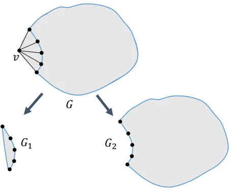
[image:4.612.192.419.72.260.2]𝑣
Figure 1: Illustration of the vertex splitting algorithm. G1 contains all neighbors of v (withoutv
itself) and the edges between them; G2 contains all vertices and edges ofGexceptvand the edges
incident tov.
latter asks for a maximum independent set of vertices ofG, that is a set such that no two vertices from it are connected by an edge in G. Specifically, an independent set of H = (V, E) defines a clique in graph G = (V, E), where E is the complement of set E. This leads to a constrained formulation of Maximum Clique given by
maximize xv∈{0,1}
X
v∈V
xv subject to X
(u,v)∈E
xuxv = 0. (3)
The constraint formulation can equivalently be written in QUBO form as
H=−AX
v∈V
xv+B X
(u,v)∈E
xuxv, (4)
where the penalty weights can be chosen as A= 1, B = 2 (Lucas, 2014). One disadvantage of (4) lies in the fact that H contains O(n2) quadratic terms for sparse graphs (ofO(n) edges), limiting the size of problems that can fit DW.
An alternative QUBO formulation of Lucas (2014) assumes the clique size K≥1 is known. Its Hamiltonian
HK=A
K−X
v∈V
xv 2
+B
K
2
− X
(u,v)∈E
xuxv
(5)
is designed to attain the value zero only for an assignment defining a clique of size K, which is achieved if one chooses weights A=K+ 1 and B = 1 (Lucas, 2014).
3.2 Problem decomposition
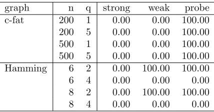
graph n q strong weak probe c-fat 200 1 0.00 0.00 100.00 200 5 0.00 0.00 100.00 500 1 0.00 0.00 100.00 500 5 0.00 0.00 100.00 Hamming 6 2 0.00 100.00 100.00 6 4 0.00 0.00 0.00 8 2 0.00 100.00 100.00 8 4 0.00 0.00 0.00
Table 1: Reduction in % from strong and weak persistencies as well as probing on selected c-fat and Hamming graphs. Qubo for maximum clique.
generated subproblem fits DW. After solving each subproblem, the solutions are combined again into a solution to Maximum Clique for the original graph.
We describe here an improved version of the most universal of those algorithms, in the sense that it can be applied to all input graphs regardless of their structure. It works as follows. Given a graphG= (V, E), pick any vertexv, e.g, with the smallest number of neighbors as in Djidjev et al. (2017), and define two new graphs: a graphG1 induced by all neighbors ofv(but without vitself)
and the graphG2 induced byV \ {v}, that isGwithout v and its incident edges (Figure 1). Then
find recursively the maximum cliquesC1 ofG1 andC2 of G2. If|C1|>|C2|, return as a maximum
clique forG the subgraph induced byC1∪ {v}, otherwise returnC2. The recursion stops whenG
is small enough to fit DW.
It is easy to see the recursion is finite, as bothG1 and G2 contain no more than|V| −1 vertices
each, since neither of them containsv, and that it correctly finds a clique of maximum size for G. Unfortunately, in the worst case it may generate an exponential number of subgraphs (exponential in the size of G). We will study in the next subsection how persistency analysis can help to reduce the number of subgraphs generated.
3.3 Results with Qpbo
In our experiments, we used the C++ package Qpbo of Rother et al. (2007); Kolmogorov (2014) for finding persistencies, developed for computer vision applications. We access Qpbo through a Python interface that we adapted by modifying the PyQpbo package (M¨uller and Behnke, 2014). This section presents results on the effectiveness of the method for Maximum Clique. We investigate the application of Qpbo to QUBOs (4) and (5) on random as well as special graphs (c-fat and Hamming graphs), both without and in connection with the graph splitting algorithm of Section 3.2. Moreover, we compare the two QUBO formulations (4) and (5) presented in Section 3.1.
3.3.1 Qpbo on c-fat and Hamming graphs
We apply Qpbo to the QUBO formulation (4). The test graphs we use are from the1993 DIMACS Challenge on maximum cliques, coloring and satisfiabilty (Johnson and Trick, 1996) and have also been used in Boros et al. (2006). Both graph families depend on two parameters: the number of verticesnand an additional internal parameter, precisely the partition parametercfor c-fat graphs and the Hamming distancedfor Hamming graphs. We use the generation algorithms of Hasselberg et al. (1993) for both graph families.
Table 1 shows the results (where both parameterscanddare summarized as a generic parameter
0.970 0.975 0.980 0.985 0.990 0.995 1.000
0.0
0.2
0.4
0.6
0.8
1.0
probability p
percentage of solv
ed v
ar
iab
les
strong weak
0.88 0.90 0.92 0.94 0.96 0.98 1.00
0.0
0.2
0.4
0.6
0.8
1.0
probability p
percentage of solv
ed v
ar
iab
les
[image:6.612.94.510.91.278.2]strong weak
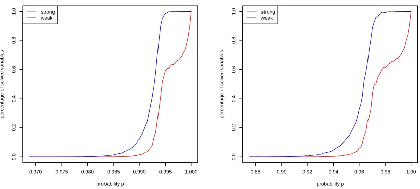
Figure 2: Percentage of found (strong and weak) persistencies with Qpbo as a function of the edge probabilitypwith which random edges are inserted. C-fat graph withn= 500 andc= 2 (left) and Hamming graph with n= 8 and d= 4 (right).
while in the remaining two cases it cannot find any persistency. Also we observe that probing is the most effective algorithm, while finding strong persistencies is the least effective.
In order to observe and compare a wider range of percentages of solved variables with Qpbo, we insert (or delete) edges from c-fat or Hamming graphs with a certain probability p which we will vary.
Figure 2 (left) shows that when adding random edges (with edge probability p) to the (500,2) c-fat graph, no strong and weak persistencies are found for both the original graph as well as for almost all dense modified graphs (since the x-axis starts atp= 0.97). Persistencies (as a percentage of solved variables out of the n= 500 variables in the QUBO) are only observed for p≥0.97 and increase to 100% over a very short range. As expected, weak persistencies are found (slightly) earlier than strong ones. The behavior for the Hamming graph withn= 8 and Hamming distance
d= 4 is similar.
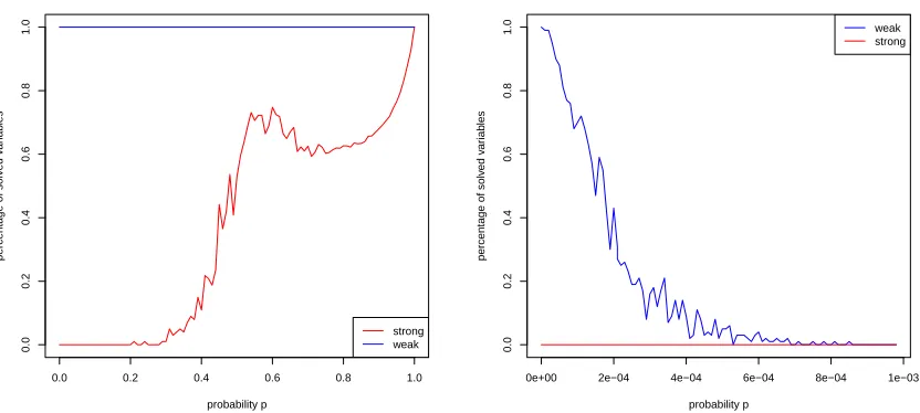
Similarly to Figure 2, Figure 3 shows strong and weak persistencies as a function of p for the Hamming graph withn= 8 andd= 4. However, the behavior of strong and weak persistencies is different in this case. Figure 3 shows that Qpbo is able to assign a value to 100% of all variables in the QUBO of the original Hamming graph via weak persistencies (see Table 1). Nevertheless, strong persistencies are not found. We therefore add edges with probabilityp to observe a progression of strong persistencies (Fig. 3, left) and remove edges with probabilitypfor weak persistencies (Fig. 3, right).
Figure 3 shows that strong persistencies increase gradually over the entire interval p ∈ [0,1], whereas the found weak persistencies disappear almost instantly as soon as edges are removed from the graph.
3.3.2 Comparison of alternative QUBO formulations for Maximum Clique
0.0 0.2 0.4 0.6 0.8 1.0
0.0
0.2
0.4
0.6
0.8
1.0
probability p
percentage of solv
ed v
ar
iab
les
strong weak
0e+00 2e−04 4e−04 6e−04 8e−04 1e−03
0.0
0.2
0.4
0.6
0.8
1.0
probability p
percentage of solv
ed v
ar
iab
les
[image:7.612.96.512.90.277.2]weak strong
Figure 3: Percentage of found (strong and weak) persistencies with Qpbo as a function of the edge probability p with which random edges are inserted (in case of strong persistencies, left plot) or deleted (in case of weak persistencies, right plot). Hamming graph with n= 8 and d= 2.
p formu- QUBO
graph n orc lation size strong weak
Ham- 8 2 (4) 1280 0 100
ming 8 2 (5) 65536 0 0
c-fat 200 1 (4) 481 69 100
[image:7.612.183.431.344.420.2]200 1 (5) 40000 0 0
Table 2: Reduction of the number of variables in percentage for the two QUBO formulations for maximal clique on Hamming and fat graphs.
parameter. Nevertheless, this section investigates whether the choice of formulation has an effect on the persistencies found and whether changing the QUBO formulation can result in more or fewer persistencies. If this is the case, then it may be worth investing time to search for formulations that are more suitable for the persistency algorithm.
In order to find the clique size that is needed for (5), we first run an alternative algorithm to find the maximum clique size K for each tested graph. We then compute the QUBO coefficients for (5) with parameterK and identify strong and weak persistencies using Qpbo.
Table 2 shows results for a Hamming graph with parametersn= 8 andd= 2 and a c-fat graph with parametersn= 200 andc= 1. As can be seen from the table, formulation (5) results in much larger QUBO problems (which are likely to also have a more complex structure, thus being more difficult to solve for Qpbo) and thus in fewer persistencies compared to (4), so clearly the latter formulation is preferable, at least for the type of graphs tested.
3.3.3 Combining Qpbo with the decomposition algorithm
●
●
●
●
●
10000 15000 20000 25000 30000 35000 40000
0.0
0.1
0.2
0.3
0.4
0.5
expected number of edges
e
xcess r
atio solv
[image:8.612.191.413.94.299.2]er calls
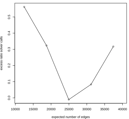
Figure 4: Proportional saving as a function of the expected number of edges of the random graph when using Qpbo in the graph splitting routine, computed as (nqpbo−nno-qpbo)/nno-qpbo, where
nqpbo and nno-qpbo denote the number of solver calls when employing graph splitting with and
without Qpbo.
prohibitively long) and, if found, reduce the size of the graph by removing the corresponding variables. We stop splitting when all generated (sub-)graphs are of size small enough to fit DW, which in our case is 45 vertices.
We test the resulting algorithm on random graphs with n = 500 vertices and an expected number of edges in the interval [10000,40000].
Figure 4 visualizes the proportional reduction in the number of generated subproblems. For this, we plot the ratio (nqpbo−nno-qpbo)/nno-qpbo as a function ofp, wherenqpboandnno-qpbodenote the
number of solver calls when employing graph splitting with and without Qpbo, respectively. The figure shows that, especially for sparse graphs, substantial reductions with respect to the number of generated subproblems can be achieved.
4
The maximum cut problem
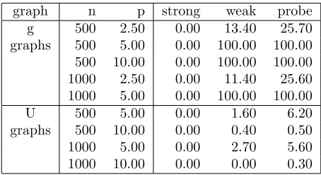
graph n p strong weak probe g 500 2.50 0.00 13.40 25.70 graphs 500 5.00 0.00 100.00 100.00 500 10.00 0.00 100.00 100.00 1000 2.50 0.00 11.40 25.60 1000 5.00 0.00 100.00 100.00 U 500 5.00 0.00 1.60 6.20 graphs 500 10.00 0.00 0.40 0.50 1000 5.00 0.00 2.70 5.60 1000 10.00 0.00 0.00 0.30
Table 3: Reduction in % from strong and weak persistencies as well as probing on selected g and U graphs. Qubo for maximum cut.
4.1 QUBO and Ising formulation
We use the QUBO formulation for Maximum Cut of Boros and Hammer (1991) who show that the valuef of any cut in a graph G= (V, E) is given as
f(x) = X
(u,v)∈E
(xu(1−xv) + (1−xu)xv), (6)
wherexu ∈ {0,1}for allu∈V is the indicator signalling which side of the cut vertexu belongs to. Maximizing (6) over x∈ {0,1}|V| leads to a maximum cut.
The formulation (6) can be simplified when switching the input range of xu to an Ising model. In (6), each term xu(1−xv) + (1−xu)xv is zero if and only ifu and v belong to the same side of the cut, and one otherwise. In an Ising formulation, that is whenxu ∈ {−1,+1}for all u∈V, the same term can be expressed as (1−xuxv)/2, leading to the Hamiltonian
H0(x) =
X
(u,v)∈E 1
2(1−xuxv),
which has to be maximized (just like (6)). Equivalently, we can minimize
H(x) =− X
(u,v)∈E
(1−xuxv) =−|E|+ X
(u,v)∈E
xuxv
∼ X
(u,v)∈E
xuxv, (7)
since|E|is constant. In the following we will solely use the simpler Ising formulation (7).
4.2 Ising on g and U graphs
We test Qpbo on the Ising formulation (7) for the Maximum Cut problem applied to g and U
Additionally, we again studied how the performance of Qpbo varies as the graph becomes denser by adding or removing random edges. These results are similar to the ones already described for Maximum Clique (Figures 2 and 3) and are thus not presented here.
5
Conclusions
This paper studies the use of preprocessing methods to reduce the size of QUBO and Ising integer programs. Such models have recently attracted increased attention since they allow constant time solutions on newly available quantum annealers. However, the small number of available qubits on such devices severely limits the range of solvable problems. This motivates the use of preprocessing methods to reduce the number of required qubits, thus extending the application range of such devices.
We use the package Qpbo (Kolmogorov, 2014; M¨uller and Behnke, 2014) to compute strong and weak persistencies in integer programs and test the suitability of preprocessing methods on two important NP-hard graph problems, the Maximum Clique and the Maximum Cut problems.
Our main findings can be summarized as follows:
1. The observed reduction in variables seems to be very problem-specific, both in terms of the QUBO/ Ising formulation considered as well as the employed test graphs. Test graphs on which Qpbo achieved 100% reductions for Maximum Clique did not lead to any reduction for Maximum Cut or vice versa. We observe 0% and 100% reductions considerably more often than reductions between those extremes.
2. When applied to a decomposition algorithm which divides up a maximum clique computation on graphs of arbitrary size into many smaller subproblems, Qpbo can be used to reduce the number of generated subproblems. This reduction seems especially significant for sparser graphs.
3. Using two different QUBO formulations for Maximum Clique, we show that the performance of Qpbo is not only dependent on the type of problem solved and the input graph, but also on the specific QUBO formulation used. This, therefore, justifies research into finding formula-tions for different optimization problems that are more suitable for identifying persistencies. This is consistent with the much more general observation in combinatorial optimization prac-tice that the choice of formulation for a given optimization problem can have a huge effect on the time it will take to solve the resulting problem using popular solvers.
The effectiveness of Qpbo varied widely between seemingly similar problem instances. An especially interesting and practically important open problem is to be able to characterize input graphs and problem formulations that are more suitable for identification of persistencies.
References
Balas, E. and Yu, C. (1986). Finding a maximum clique in an arbitrary graph. SIAM J Comp, 15:1054–1068.
Boros, E. and Hammer, P. (1991). The max-cut problem and quadratic 0-1 optimization; Polyhedral aspects, relaxations and bounds. Ann Oper Res, 33:151–180.
Boros, E. and Hammer, P. (2001). Pseudo-Boolean Optimization. Rutcor Report, pages 1–83.
Boros, E., Hammer, P., and Tavares, G. (2006). Preprocessing of Unconstrained Quadratic Binary Optimization. Rutcor Research Report, RRR 10-2006:1–58.
Bunyk, P., Hoskinson, E., Johnson, M., Tolkacheva, E., Altomare, F., Berkley, A., Harris, R., Hilton, J., Lanting, T., Przybysz, A., and Whittaker, J. (2014). Architectural considerations in the design of a superconducting quantum annealing processor. IEEE Trans on Appl Supercon-ductivity, 24(4):1–10.
D-Wave (2016). Introduction to the D-Wave quantum hardware.
Djidjev, H., Chapuis, G., Hahn, G., and Rizk, G. (2017). Finding maximum cliques on a quantum annealer. ACM Computing Frontiers, 1(1):1–8.
Hammer, P., Hansen, P., and Simeone, B. (1984). Roof duality, complementation and persistency in quadratic 0-1 optimization. Mathematical Programming, 28(2):121–155.
Hasselberg, J., Pardalos, P., and Vairaktarakis, G. (1993). Test Case Generators and Computational Results for the Maximum Clique Problem. Journal of Global Optimization, 3:463–482.
Johnson, D. and Trick, M., editors (1996). Clique, Coloring, and Satisfiability: Second DIMACS Implementation Challenge, DIMACS, volume 26. American Mathematical Society.
Johnson, M., Amin, M., Gildert, S., Lanting, T. Hamze, F., Dickson, N., Harris, R., Berkley, A., Johansson, J., Bunyk, P., Chapple, E., Enderud, C., Hilton, J., Karimi, K., Ladizinsky, E., Ladizinsky, N., Oh, T., Perminov, I., Rich, C., Thom, M., Tolkacheva, E., Truncik, C., Uchaikin, S., Wang, J., B., W., and Rose, G. (2011). Quantum annealing with manufactured spins. Nature, 473:194–198.
Kim, S.-H., Kim, Y.-H., and Moon, B.-R. (2001). A Hybrid Genetic Algorithm for the MAX CUT Problem. Proceeding GECCO’01 Proceedings of the 3rd Annual Conference on Genetic and Evolutionary Computation, pages 416–423.
King, J., Yarkoni, S., Nevisi, M. M., Hilton, J. P., and McGeoch, C. C. (2015). Benchmarking a quantum annealing processor with the time-to-target metric. arXiv:1508.05087, pages 1–29.
Kolmogorov, V. (2014). QPBO v1.4 software package. C++ package manual.
Lucas, A. (2014). Ising formulations of many np problems. Frontiers in Physics, 2(5):1–27.
M¨uller, A. C. and Behnke, S. (2014). Pystruct - Learning Structured Prediction in Python. Journal of Machine Learning Research, 15:2055–2060.