Reducing Dimensions of Tensors in Type Driven Distributional Semantics

Reducing Dimensions of Tensors in Type-Driven Distributional Semantics

Tamara Polajnar Luana Fˇagˇarˇas¸an Stephen Clark

Computer Laboratory University of Cambridge

Cambridge, UK

first.last@cl.cam.ac.uk

Abstract

Compositional distributional semantics is a subfield of Computational Linguistics which investigates methods for represent-ing the meanrepresent-ings of phrases and sen-tences. In this paper, we explore im-plementations of a framework based on Combinatory Categorial Grammar (CCG), in which words with certain grammatical types have meanings represented by multi-linear maps (i.e. multi-dimensional arrays, or tensors). An obstacle to full implemen-tation of the framework is the size of these tensors. We examine the performance of lower dimensional approximations of tran-sitive verb tensors on a sentence plausi-bility/selectional preference task. We find that the matrices perform as well as, and sometimes even better than, full tensors, allowing a reduction in the number of pa-rameters needed to model the framework.

1 Introduction

An emerging subfield of computational linguis-tics is concerned with learning compositional dis-tributional representations of meaning (Mitchell and Lapata, 2008; Baroni and Zamparelli, 2010; Coecke et al., 2010; Grefenstette and Sadrzadeh, 2011; Clarke, 2012; Socher et al., 2012; Clark, 2013). The advantage of such representations lies in their potential to combine the benefits of dis-tributional approachs to word meaning (Sch¨utze, 1998; Turney and Pantel, 2010) with the more tra-ditional compositional methods from formal se-mantics (Dowty et al., 1981). Distributional repre-sentations have the properties of robustness, learn-ability from data, ease of handling ambiguity, and the ability to represent gradations of mean-ing; whereas compositional models handle the un-bounded nature of natural language, as well as

providing established accounts of logical words, quantification, and inference.

One promising approach which attempts to combine elements of compositional and distribu-tional semantics is by Coecke et al. (2010). The underlying idea is to take the type-driven approach from formal semantics — in particular the idea that the meanings of complex grammatical types should be represented as functions — and ap-ply it to distributional representations. Since the mathematics of distributional semantics is pro-vided by linear algebra, a natural set of functions to consider is the set of linear maps. Coecke et al. recognize that there is a natural correspon-dence from complex grammatical types to tensors (multi-linear maps), so that the meaning of an ad-jective, for example, is represented by a matrix (a 2nd-order tensor)1_{and the meaning of a transitive}

verb is represented by a 3rd-order tensor.

Coecke et al. use the grammar of pregroups as the syntactic machinery to construct distribu-tional meaning representations, since both pre-groups and vector spaces can be seen as exam-ples of the same abstract structure, which leads to a particularly clean mathematical description of the compositional process. However, the approach applies more generally, for example to other forms of categorial grammar, such as Combinatory Cate-gorial Grammar (Steedman, 2000; Maillard et al., 2014), and also to phrase-structure grammars in a way that a formal linguist would recognize (Ba-roni et al., 2014). Clark (2013) provides a descrip-tion of the tensor-based framework aimed more at computational linguists, relying only on the math-ematics of multi-linear algebra rather than the cat-egory theory used in Coecke et al. (2010). Sec-tion 2 repeats some of this descripSec-tion.

A major open question associated with the tensor-based semantic framework is how to learn

1_{This same insight lies behind the work of Baroni and} Zamparelli (2010).

the tensors representing the meanings of words with complex types, such as verbs and adjec-tives. The framework is essentially a composi-tional framework, providing a recipe for how to combine distributional representations, but leav-ing open what the underlyleav-ing vector spaces are and how they can be acquired. One significant chal-lenge is an engineering one: in a wide-coverage grammar, which is able to handle naturally occur-ring text, there will be a) a large lexicon with many word-category pairs requiring tensor representa-tions; and b) many higher-order tensors with large numbers of parameters which need to be learned. In this paper we take a first step towards learning such representations, by learning tensors for tran-sitive verbs.

One feature of the tensor-based framework is that it allows the meanings of words and phrases with different basic types, for example nouns and sentences, to live in different vector spaces. This means that the sentence space is task specific, and must be defined in advance. For example, to calcu-late sentence similarity, we would have to learn a vector space where distances between vectors rep-resenting the meanings of sentences reflect simi-larity scores assigned by human annotators.

In this paper we describe an initial investi-gation into the learning of word meanings with complex syntactic types, together with a simple sentence space. The space we consider is the “plausibility space” described by Clark (2013), to-gether with sentences of the form subject-verb-object. This space is defined to distinguish se-mantically plausible sentences (e.g. Animals eat plants) from implausible ones (e.g. Animals eat planets). Plausibility can be either represented as a single continuous variable between 0 and 1, or as a two-dimensional probability distribution over the classesplausible(>) andimplausible(⊥). Whether we consider a one- or two-dimensional sentence space depends on the architecture of the logistic regression classifier that is used to learn the verb (Section 3).

We begin with this simple plausibility sentence space to determine if, in fact, the tensor-based rep-resentation can be learned to a sufficiently useful degree. Other simple sentence spaces which can perhaps be represented using one or two variables include a “sentence space” for the sentiment anal-ysis task (Socher et al., 2013), where one variable represents positive sentiment and the other

nega-tive. We also expect that the insights gained from research on this task can be applied to more com-plex sentence spaces, for example a semantic simi-larity space which will require more than two vari-ables.

2 Syntactic Types to Tensors

The syntactic type of a transitive verb in English is (S\NP)/NP (using notation from Steedman (2000)), meaning that a transitive verb is a func-tion which takes anNP argument to the right, an

NP argument to the left, and results in a sentence

S. Suchcategorieswith slashes arecomplex cate-gories;S andNP arebasicoratomiccategories. Interpreting such categories under the Coecke et al. framework is straightforward. First, for each atomic category there is a corresponding vector space; in this case the sentence space S and the noun spaceN.2 _{Hence the meaning of a noun or}

noun phrase, for examplepeople, will be a vector in the noun space:−−−→people∈N. In order to obtain the meaning of a transitive verb, each slash is re-placed with a tensor product operator, so that the meaning ofeat, for example, is a 3rd-order tensor:

eat ∈ S⊗N⊗N. Just as in the syntactic case, the meaning of a transitive verb is a function (a multi-linear map) which takes two noun vectors as arguments and returns a sentence vector.

Meanings combine using tensor contraction, which can be thought of as a multi-linear gen-eralisation of matrix multiplication (Grefenstette, 2013). Consider first the adjective-noun case, for example black cat. The syntactic type of black

isN/N; hence its meaning is a 2nd-order tensor (matrix): black ∈ N⊗N. In the syntax, N/N

combines withN using the rule of forward appli-cation (N/N N ⇒ N), which is an instance of function application. Function application is also used in the tensor-based semantics, which, for a matrix and vector argument, corresponds to ma-trix multiplication.

Figure 1 shows how the syntactic types com-bine with a transitive verb, and the corresponding tensor-based semantic types. Note that, after the verb has combined with its object NP, the type of the verb phrase is S\NP, with a correspond-ing meancorrespond-ing tensor (matrix) inS⊗N. This ma-trix then combines with the subject vector, through

people eat fish NP (S\NP)/NP NP

N S⊗N⊗N N

>

S\NP

S⊗N

<

S

S

Figure 1: Syntactic reduction and tensor-based se-mantic types for a transitive verb sentence

matrix multiplication, to give a sentence vector. In practice, using for example the wide-coverage grammar from CCGbank (Hockenmaier and Steedman, 2007), there will be many types with more than 3 slashes, with corresponding higher-order tensors. For example, a com-mon category for a preposition is the follow-ing: ((S\NP)\(S\NP))/NP, which would be assigned to WITHin eat WITHa fork. (The way

to read the syntactic type is as follows: with re-quires an NP argument to the right – a fork in this example – and then a verb phrase to the left – eat with type S\NP – resulting in a verb phraseS\NP.) The corresponding meaning ten-sor lives in the tenten-sor spaceS⊗N⊗S⊗N⊗N, i.e. a 5th-order tensor. Categories with even more slashes are not uncommon, for example ((N/N)/(N/N))/((N/N)/(N/N)). Clearly learning parameters for such tensors is highly challenging, and it is likely that lower dimensional approximations will be required.

3 Methods

In this paper we compare five different methods for modelling the type-driven semantic represen-tation of subject-verb-object sentences. The ten-sor is a function that encodes the meaning of a verb. It takes two vectors from theK-dimensional noun space as input, and produces a representa-tion of the sentence in theS-dimensional sentence space. In this paper, we consider a plausibility spacewhereSis either a single variable or a two-dimensional space over two classes:plausible(>) andimplausible(⊥).

The first method (Tensor) follows Krishna-murthy and Mitchell (2013) by learning a tensor as parameters in a softmax classifier. We introduce three related methods (2Mat, SKMat, KKMat), all of which model the verb as a matrix or a pair of matrices (Figure 2). Table 1 gives the number of

Tensor 2Mat SKMat KKMat DMat

V 2K2 _{4K 2K K}2 _K2

Θ 4 8 4 0 0

Table 1: Number of parameters per method.

parameters for each method. Tensor, 2Mat, and SKMatall have a two-dimensionalSspace, while KKMatproduces a scalar value. In all of these learning-based methods the derivatives were ob-tained via the chain rule with respect to each set of parameters and gradient descent was performed using the Adagrad algorithm (Duchi et al., 2011).

We also reimplement a distributional method (DMat), which was previously used in SVO experiments with the type-driven framework (Grefenstette and Sadrzadeh, 2011). While the other methods are trained as plausibility classi-fiers, in DMat we estimate the class boundary from cosine similarity via training data (see expla-nation below).

Tensor If subject (ns) and object (no) nouns are

K-dimensional vectors and the plausibility vec-tor is S-dimensional with S = 2, we can learn the values of the K ×K ×S tensor represent-ing the verb as parameters (V) of a regression al-gorithm. To represent this space as a distribution over two classes (>,⊥) we apply a sigmoid func-tion (σ) to restrict the output to the [0,1] range and the softmax activation function (g) to balance the class probabilities. The full parameter set which needs to be optimised for isB = {V,Θ}, where Θ = {θ>, θ⊥} are the softmax parameters for the two classes. For each verb we optimise the KL-divergence L between the training labels ti and classifier predictions using the following reg-ularised objective:

O(B) =XN

i=1

L ti_{, g}

σ hV

ni

s, nio

,Θ

+λ₂||B||2

(1)

where ni

s and nio are the subject and object of the training instance i ∈ N, and hV nis, nio

= (ni

K

௦ ௜

௢ ௜ ்

S

K K

K

S

(a)

K

௦ ௜

௢ ௜ ்

K

S

K S

K

2*S

x

S S

x

(b)

K ௦ ௜

௢ ௜

K S

K

K

0

0 0

0

0 0

K

S

S

x

x

(c)

K

௦ ௜

௢ ௜ ்

K K

K

x x

(d)

Figure 2: Illustrations of thehVfunction for the regression-based methods(a)-Tensor, (b)-2Mat, (c) -SKMat, (d)-KKMat. The operation in(a) is tensor contraction, T denotes transpose, and×denotes matrix multiplication.

The gold-standard distribution over training labels is defined as(1,0)or(0,1), depending on whether the training instance is a positive (plausible) or negative (implausible) example. Tensor contrac-tion is implemented using the Matlab Tensor Tool-box (Bader et al., 2012).

2Mat An alternative approach is to decouple the interaction between the object and subject by learning a pair of S ×K (S = 2) matrices (Vs, Vo) for each of the input noun vectors (one ma-trix for the subject slot of the verb and one for the object slot). The resultingS-vectors are concate-nated, after the subject and object nouns have been combined with their matrices, and combined with the softmax component to produce the output dis-tribution. Therefore the objective function is the same as in Equation 1, buthVis defined as:

hV nis, nio

= (ni_s)V_sT|| Vo(nio)T _T

where||represents vector concatenation. The in-tention is to test whether we can learn the verb without directly multiplying subject and object features,ni

sandnjo. The functionhVis shown in Figure 2-(b), where the verb tensor parameters are

drawn as two2×K matrices, one of which inter-acts with the subject and the other with the object noun vector. The output is a four-dimensional vec-tor whose values are then restricted to [0,1] using the sigmoid function and then transformed into a two-dimensional distribution over the classes us-ing the softmax function.

SKMat A third option for generating a sentence vector with S = 2dimensions is to consider the verb as anS×K matrix. If we transform the ob-ject vector into aK×Kmatrix with the noun on the diagonal and zeroes elsewhere, we can com-bine the verb and object to produce a newS×K

matrix, which is encoding the meaning of the verb phrase. We can then complete the sentence re-duction by multiplying the subject vector with this verb phrase vector to produce an S-dimensional sentence vector. Formally, we defineSKMatas:

hV nis, nio=nis Vdiag(nio)T

ma-trix. The graphic demonstrates the two-step com-bination and the intermediateS×K verb phrase matrix, as well as the the noun vector product that results in a two-dimensional vector which is then transformed using the sigmoid and softmax functions. Whilst the tensor method captures the interactions between all pairs of context features (nsi·noj),SKMatonly captures the interactions between matching features (nsi·noi).

KKMat Given a two-class problem, such as

plausibility classification, the softmax implemen-tation is overparameterised because the class membership can be estimated with a single vari-able. To produce a scalar output, we can learn the parameters for a singleK ×K matrix (V) using standard logistic regression with the mean squared error cost function:

O(V) =−1 m

"_N X

i=1

tiloghV

nis, nio

+ (1−ti) loghV

nis, nio

#

wherehV nis, nio

= (ni

s)V(nio)T and the objec-tive is regularised:O(V) +λ₂||V||2_{. This function} is shown in Figure 2-(d), where the verb parame-ters are shown as a matrix, while the subject and object are vectors. The output is a single scalar, which is then transformed with the sigmoid func-tion. Values over 0.5 are considered plausible. DMat The final method produces a scalar as in KKMat, but is distributional and based on corpus counts rather than regression-based. Grefenstette and Sadrzadeh (2011) introduced a corpus-based approach for generating aK×Kmatrix for each verb from an average of Kronecker products of the subject and object vectors from the positively la-belled subset of the training data. The intuition is that, for example, the matrix foreat may have a high value for the contextual topic pair describing animate subjects and edible objects. To determine the plausibility of a new subject-object pair for a particular verb, we calculate the Kronecker prod-uct of the subject and object noun vectors for this pair, and compare the resulting matrix with the av-erage verb matrix using cosine similarity.

For label prediction, we calculate the similar-ity between each of the training data pairs and the learned average matrix. Unlike for KKmat, the class cutoff is estimated at the break-even point of the receiver operator characteristic (ROC) gen-erated by comparing the training labels with this

cosine similarity value. The break-even point is when the true positive rate is equal to the false pos-itive rate. In practice it would be more accurate to estimate the cutoff on a validation dataset, but some of the verbs have so few training instances that this was not possible.

4 Experiments

In order to examine the quality of learning we run several experiments where we compare the differ-ent methods. In these experimdiffer-ents we consider the DMat method as the baseline. Some of the experiments employ cross-validation, in particular five repetitions of 2-fold cross validation (5x2cv), which has been shown to be statistically more ro-bust than the traditional 10-fold cross validation (Alpaydin, 1999; Ulas¸ et al., 2012). The results of 5x2cv experiments can be compared using the reg-ular paired t-test, but the specially designed 5x2cv F-test has been proven to produce fewer statistical errors (Ulas¸ et al., 2012).

The performance was evaluated using the area under the ROC (AUC) and the F1 measure (based on precision and recall over the plausible class). The AUC evaluates whether a method is ranking positive examples above negative ones, regardless of the class cutoff value. F1shows how accurately a method assigns the correct class label. Another way to interpret the results is to consider the AUC as the measure of the quality of the parameters in the verb matrix or tensor, while the F-score indi-cates how well the softmax, the sigmoid, and the DMatcutoff algorithm are estimating class partic-ipation.

Ex-1. In the first experiment, we compare the different transitive verb representations by running 5x2cv experiments on ten verbs chosen to cover a range of concreteness and frequency values (Sec-tion 4.2).

Ex-2. In the initial experiments we found that some models had low performance, so we applied the column normalisation technique, which is of-ten used with regression learning to standardise the numerical range of features:

~x:= _max(~x−_~x)min(_−min(~x) _~x) (2)

Ex-3. There are varying numbers of training ex-amples for each of the verbs, so we repeated the 5x2cv with datasets of 52 training points for each verb, since this is the size of the smallest dataset of the verbCENSOR. The points were randomly

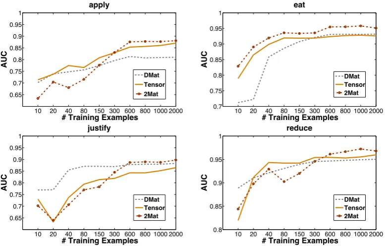
sam-pled from the datasets used in the first experiment. Finally, the four verbs with the largest datasets were used to examine how the performance of the methods changes as the amount of training data increases. The 4,000 training samples were ran-domised and half were used for testing. We sam-pled between 10 and 1000 training triples from the other half (Figure 4).

4.1 Noun vectors

Distributional semantic models (Turney and Pan-tel, 2010) encode word meaning in a vector for-mat by counting co-occurrences with other words within a specified context window. We con-structed the vectors from the October 2013 dump of Wikipedia articles, which was tokenised us-ing the Stanford NLP tools3_{, lemmatised with the}

Morpha lemmatiser (Minnen et al., 2001), and parsed with the C&C parser (Clark and Curran, 2007). In this paper we use sentence boundaries to define context windows and the top 10,000 most frequent lemmatised words in the whole corpus (excluding stopwords) as context words. The raw co-occurrence counts are re-weighted using the standard tTest weighting scheme (Curran, 2004), wherefwicj is the number of times target nounwi occurs with context wordcj:

tT est(w~i, cj) = p(wip, cj_p)_(w−p(wi)p(cj) i)p(cj) (3)

wherep(wi) = P

jfwicj P

kPlfwkcl,p(cj) = P

ifwicj P

kPlfwkcl, andp(wi, cj) = P fwicj

kPlfwkcl.

Using all 10,000 context words would result in a large number of parameters for each verb ten-sor, and so we apply singular value decomposition (SVD) (Turney and Pantel, 2010) with 40 latent dimensions to the target-context word matrix. We use context selection (with N = 140) and row normalisation as described in Polajnar and Clark (2014) to markedly improve the performance of SVD on smaller dimensions (K) and enable us to train the verb tensors using very low-dimensional

3_{http://nlp.stanford.edu/software/index.shtml}

Verb Concreteness # of Positive Frequency

APPLY 2.5 5618 47361762

CENSOR 3 26 278525

COMB 5 164 644447

DEPOSE 2.5 118 874463

EAT 4.44 5067 26396728

IDEALIZE 1.17 99 485580 INCUBATE 3.5 82 833621 JUSTIFY 1.45 5636 10517616 REDUCE 2 26917 40336784

WIPE 4 1090 6348595

Table 2: The 10 chosen verbs together with their concreteness scores. The number of positive SVO examples was capped at 2000. Frequencyis the frequency of the verb in the GSN corpus.

noun vectors. Performance of the noun vectors was measured on standard word similarity datasets and the results were comparable to those reported by Polajnar and Clark (2014).

4.2 Training data

In order to generate training data we made use of two large corpora: the Google Syntactic N-grams (GSN) (Goldberg and Orwant, 2013) and the Wikipedia October 2013 dump. We first chose ten transitive verbs with different concreteness scores (Brysbaert et al., 2013) and frequencies, in order to obtain a variety of verb types. Then the positive (plausible) SVO examples were extracted from the GSN corpus. More precisely, we col-lected all distinct syntactic trigrams of the form

nsubj ROOT dobj, where the root of the phrase was one of our target verbs. We lemmatised the words using the NLTK4_{lemmatiser and filtered these}

ex-amples to retain only the ones that contain nouns that also occur in Wikipedia, obtaining the counts reported in Table 2.

For every positive training example, we con-structed a negative (implausible) one by replac-ing both the subject and the object with a con-founder, using a standard technique from the se-lectional preference literature (Chambers and Ju-rafsky, 2010). A confounder was generated by choosing a random noun from the same frequency bucket as the original noun.5 _{Frequency buckets}

of size 10 were constructed by collecting noun fre-quency counts from the Wikipedia corpus. For

ex-4_{http://nltk.org/}

Verb Tensor DMat KKMat SKMat 2Mat AUC

APPLY 85.68† 81.46‡ 88.88†‡ 68.02 88.92†‡

CENSOR 79.40 85.54 80.55 78.52 83.19

COMB 89.41 85.65 88.38 69.20†‡ 89.56 DEPOSE 92.70 94.44 93.12 84.47† 93.20

EAT 94.62 93.81 95.17 67.92 95.88‡

IDEALIZE 69.56 75.84 72.46 61.19 70.23 INCUBATE 89.33 85.53 88.61 70.59 91.40 JUSTIFY 85.27† 88.70‡ 89.97‡ 73.56 90.10‡ REDUCE 96.13 95.48 96.69† 79.32 97.21 WIPE 85.19 84.47 87.84† 64.93†‡ 81.29

MEAN 86.93 87.29 88.37 71.96 88.30

Tensor DMat KKMat SKMat 2Mat

F1

79.27 64.00 81.24‡ 54.06 80.80‡ 70.66 47.93 73.52 37.86 71.07 81.15 45.02 81.38 39.67 82.36

84.60 54.77 84.79 43.79 86.15

88.91 52.45 88.83 56.22 89.95

66.53 48.28 68.39 31.03 67.43 80.30 50.84 80.90 31.99 84.55

79.73 73.71 81.10 54.09 82.52

91.24 71.24‡ 87.46 76.67‡ 92.22

78.57 47.62 80.65 39.50 78.90

80.30 55.79 81.03 46.69 81.79

Table 3: The best AUC and F1results for all the verbs, where†denotes statistical significance compared toDMatand‡denotes significance compared toTensoraccording to the 5x2cv F-test withp <0.05.

ample, for the plausible triple animal EAT plant,

we generate the implausible triple mountainEAT product. Some verbs were well represented in the corpus, so we used up to the top 2,000 most fre-quent triples for training.

0 0.5 1

AUC

APPLY

CENSOR COMBDEPOSE EAT

IDEALIZE_INCUBATEJUSTIFYREDUCE WIPE

Tensor Tensor* SKMat SKMat*

−0.2 0 0.2 0.4 0.6 0.8 1 1.2

F

−

Score

APPLY

CENSOR COMBDEPOSE EAT

IDEALIZE_INCUBATEJUSTIFYREDUCE WIPE

Tensor Tensor* SKMat SKMat*

Figure 3: The effect of column normalisation (*) onTensorandSKMat. Top table shows AUC and the bottom F1-score, while the error bars indicate standard deviation.

5 Results

The results from Ex-1 are summarised in Ta-ble 3. We can see that linear regression can lead

to models that are able to distinguish between plausible and implausible SVO triples. The Ten-sor method outperforms DMat, which was pre-viously shown to produce reasonable verb repre-sentations in related experiments (Grefenstette and Sadrzadeh, 2011). 2Mat and KKMat, in turn, outperform Tensor demonstrating that it is pos-sible to learn lower dimensional approximations of the tensor-based framework.2Matis an appro-priate approximation for functions with two inputs and a sentence space of any dimensionality, while KKMat is only appropriate for a single valued sentence space, such as the plausibility or senti-ment space. Due to method variance and dataset size there are very few AUC results that are sig-nificantly better than DMat and even fewer that outperformTensor. All methods perform poorly on the verb IDEALIZE, probably because it has

the lowest concreteness value and is in one of the smallest datasets. This verb is also particularly dif-ficult because it does not select strongly for either its subject or object, and so some of the pseudo-negative examples are in fact somewhat plausible (e.g. townIDEALIZEauthorityorchild IDEALIZE racehorse). In general, this would indicate that more concrete verbs are easier to learn, as they have a clearer pattern of preferred property types, but there is no distinct correlation.

Verb Tensor DMat KKMat SKMat 2Mat AUC

APPLY 86.16† 48.63‡ 82.63†‡ 85.73† 85.65†

CENSOR 75.74 71.20 78.00 82.77 78.64

COMB 91.67† 62.42‡ 90.85† 89.79† 91.42†

DEPOSE 93.96† 54.93‡ 93.56† 93.87† 93.81†

EAT 95.64† 47.68‡ 92.92† 94.99†‡ 94.76†

IDEALIZE 69.64 55.98 72.20†‡ 76.71†‡ 71.85† INCUBATE 90.97† 61.31‡ 89.69† 90.19† 90.05† JUSTIFY 89.76† 54.87‡ 87.26†‡ 89.64† 89.05† REDUCE 96.63† 59.58‡ 94.99†‡ 96.14† 96.53†

WIPE 86.82† 58.02‡ 84.18† 83.65† 86.02†

MEAN 87.90 57.66 86.83 88.55 87.98

Tensor DMat KKMat SKMat 2Mat

F1

45.57 46.99 46.17 60.86 76.60† 30.43 55.16 65.19 49.59 44.22 33.37 61.05 71.20 64.56 75.96 42.73 39.71 73.07 54.51 56.54 60.42 47.42 58.80 69.05 87.44† 39.14 49.16 41.75 31.57 50.59

46.35 53.33 70.45 41.57 63.61 47.38 51.40 41.91 63.96 80.55† 51.63 54.27 69.18 69.76 90.77† 44.04 55.19 47.84 49.89 75.80

44.31 51.57 58.76 55.73 70.41

Table 4: The best AUC and F1results for all the verbs with normalised vectors, where†denotes statistical significance compared toDMatand‡denotes significance compared toTensoraccording to the 5x2cv F-test withp <0.05.

Figure 3. This figure also shows that AUC values have much lower variance, but that high variance in F-score leads to results that are not statistically significant.

When considering the size of the datasets ( Ex-3), it would seem from Table 5 that2Matis able to learn from less data thanDMatorTensor. While this may be true over a 5x2cv experiment on small data, Figure 4 shows that this view may be overly simplistic and that different training examples can influence learning. Analysis of errors shows that the baseline method mostly generates false nega-tive errors (i.e. predicting implausible when the gold standard label is plausible). In contrast, Ten-sorproduces almost equal numbers of false posi-tives and false negaposi-tives, but sometimes produces false negatives with low frequency nouns (e.g.

bourgeoisieIDEALIZEwork), presumably because

there is not enough information in the noun vec-tor to decide on the correct class. It also produces some false positive errors when either of the nouns is plausible (but the triple is implausible), which would suggest results may be improved by train-ing with data where only one noun is confounded or by treating negative data as possibly positive (Lee and Liu, 2003).

6 Discussion

Current methods which derive distributed repre-sentations for phrases, for example the work of Socher et al. (2012), typically use only matrix rep-resentations, and also assume that words, phrases and sentences all live in the same vector space. The tensor-based semantic framework is more flexible, in that it allows different spaces for dif-ferent grammatical types, which results from it

be-Verb Tensor DMat 2Mat

APPLY 95.76 86.50 86.31 CENSOR 82.97 84.09 77.79 COMB 90.13 92.93 95.18 DEPOSE 92.41 91.27 95.61

EAT 99.64 98.25 99.58

IDEALIZE 75.03 76.68 88.98 INCUBATE 91.10 87.20 96.42

JUSTIFY 88.96 88.99 87.31

REDUCE 100.0 99.87 99.46

WIPE 97.20 91.63 96.36

MEAN 91.52 89.94 92.50

Table 5: Results show average of 5x2cv AUC on small data (26 positive + 26 negative per verb). None of the results are significant.

ing tied more closely to a type-driven syntactic de-scription; however, this flexibility comes at a cost, since there are many more paramaters to learn.

Various communities are beginning to recog-nize the additional power that tensor representa-tions can provide, through the capturing of interac-tions that are difficult to represent with vectors and matrices (see e.g. (Ranzato et al., 2010; Sutskever et al., 2009; Van de Cruys et al., 2012)). Hierar-chical recursive structures in language potentially represent a large number of such interactions – the obvious example for this paper being the interac-tion between a transitive verb’s subject and object – and present a significant challenge for machine learning.

10 20 40 80 150 300 600 800 1000 2000 0.65

0.7 0.75 0.8 0.85 0.9 0.95 1

# Training Examples

AUC

apply

DMat Tensor 2Mat

10 20 40 80 150 300 600 800 1000 2000

0.7 0.75 0.8 0.85 0.9 0.95 1

# Training Examples

AUC

eat

DMat Tensor 2Mat

10 20 40 80 150 300 600 800 1000 2000

0.65 0.7 0.75 0.8 0.85 0.9 0.95 1

# Training Examples

AUC

justify

DMat Tensor 2Mat

10 20 40 80 150 300 600 800 1000 2000 0.8

0.85 0.9 0.95 1

# Training Examples

AUC

reduce

DMat Tensor 2Mat

Figure 4: Comparison ofDMat, Tensor, and 2Mat methods as the number of training instances in-creases.

logic examples. Here, we go beyond this by learn-ing tensors uslearn-ing corpus data and by derivlearn-ing sev-eral different matrix representations for the verb in the subject-verb-object (SVO) sentence.

This work can also be thought of as applying neural network learning techniques to the clas-sic problem of selectional preference acquisition, since the design of the pseudo-disambiguation ex-periments is taken from the literature on selec-tional preferences (Clark and Weir, 2002; Cham-bers and Jurafsky, 2010). We do not compare di-rectly with methods from this literature, e.g. those based on WordNet (Resnik, 1996; Clark and Weir, 2002) or topic modelling techniques (Seaghdha, 2010), since our goal in this paper is not to ex-tend the state-of-the-art in that area, but rather to use selectional preference acquisition as a test bed for the tensor-based semantic framework.

7 Conclusion

In this paper we introduced three dimensionally reduced representations of the transitive verb ten-sor defined in the type-driven framework for com-positional distributional semantics (Coecke et al., 2010). In a comprehensive experiment on ten dif-ferent verbs we find no significant difference be-tween the full tensor representation and the re-duced representations. TheSKMatand2Mat

rep-resentations have the lowest number of parame-ters and offer a promising avenue of research for more complex sentence structures and sentence spaces. KKMatandDMatalso had high scores on some verbs, but these representations are appli-cable only in spaces where a single-value output is appropriate.

In experiments where we varied the amount of training data, we found that in general more crete verbs can learn from less data. Low con-creteness verbs require particular care with dataset design, since some of the seemingly random ex-amples can be plausible. This problem may be circumvented by using semi-supervised learning techniques.

References

Ethem Alpaydin. 1999. Combined 5x2 CV F-test for comparing supervised classification learning al-gorithms. Neural Computation, 11(8):1885–1892, November.

Brett W. Bader, Tamara G. Kolda, et al. 2012. Matlab tensor toolbox version 2.5. Available online, Jan. Marco Baroni and Roberto Zamparelli. 2010. Nouns

are vectors, adjectives are matrices: Representing adjective-noun constructions in semantic space. In

Conference on Empirical Methods in Natural Lan-guage Processing (EMNLP-10), pages 1183–1193, Cambridge, MA.

Marco Baroni, Raffaella Bernardi, and Roberto Zam-parelli. 2014. Frege in space: A program for com-positional distributional semantics. Linguistic Is-sues in Language Technology, 9:5–110.

Marc Brysbaert, Amy Beth Warriner, and Victor Ku-perman. 2013. Concreteness ratings for 40 thou-sand generally known English word lemmas. Be-havior research methods, pages 1–8.

Nathanael Chambers and Dan Jurafsky. 2010. Im-proving the use of pseudo-words for evaluating se-lectional preferences. InProceedings of ACL 2010, Uppsala, Sweden.

Stephen Clark and James R. Curran. 2007. Wide-coverage efficient statistical parsing with CCG and log-linear models. Computational Linguistics, 33(4):493–552.

Stephen Clark and David Weir. 2002. Class-based probability estimation using a semantic hierarchy.

Computational Linguistics, 28(2):187–206.

Stephen Clark. 2013. Type-driven syntax and seman-tics for composing meaning vectors. In Chris He-unen, Mehrnoosh Sadrzadeh, and Edward Grefen-stette, editors, Quantum Physics and Linguistics: A Compositional, Diagrammatic Discourse, pages 359–377. Oxford University Press.

Daoud Clarke. 2012. A context-theoretic frame-work for compositionality in distributional seman-tics. Computational Linguistics, 38(1):41–71.

Bob Coecke, Mehrnoosh Sadrzadeh, and Stephen Clark. 2010. Mathematical foundations for a com-positional distributional model of meaning. In J. van Bentham, M. Moortgat, and W. Buszkowski, edi-tors, Linguistic Analysis (Lambek Festschrift), vol-ume 36, pages 345–384.

James R. Curran. 2004. From Distributional to Seman-tic Similarity. Ph.D. thesis, University of Edinburgh. David R. Dowty, Robert E. Wall, and Stanley Peters. 1981. Introduction to Montague Semantics. Dor-drecht.

John Duchi, Elad Hazan, and Yoram Singer. 2011. Adaptive subgradient methods for online learning and stochastic optimization. J. Mach. Learn. Res., 12:2121–2159, July.

Yoav Goldberg and Jon Orwant. 2013. A dataset of syntactic-ngrams over time from a very large corpus of English books. In Second Joint Conference on Lexical and Computational Semantics, pages 241– 247, Atlanta,Georgia.

Edward Grefenstette and Mehrnoosh Sadrzadeh. 2011. Experimental support for a categorical composi-tional distribucomposi-tional model of meaning. In Proceed-ings of the 2011 Conference on Empirical Methods in Natural Language Processing, pages 1394–1404, Edinburgh, Scotland, UK, July.

Edward Grefenstette, Georgiana Dinu, Yao-Zhong Zhang, Mehrnoosh Sadrzadeh, and Marco Baroni. 2013. Multi-step regression learning for compo-sitional distributional semantics. Proceedings of the 10th International Conference on Computational Semantics (IWCS 2013).

Edward Grefenstette. 2013. Category-Theoretic Quantitative Compositional Distributional Models of Natural Language Semantics. Ph.D. thesis, Uni-versity of Oxford.

Julia Hockenmaier and Mark Steedman. 2007. CCG-bank: a corpus of CCG derivations and dependency structures extracted from the Penn Treebank. Com-putational Linguistics, 33(3):355–396.

Jayant Krishnamurthy and Tom M Mitchell. 2013. Vector space semantic parsing: A framework for compositional vector space models. In Proceed-ings of the 2013 ACL Workshop on Continuous Vec-tor Space Models and their Compositionality, Sofia, Bulgaria.

Wee Sun Lee and Bing Liu. 2003. Learning with posi-tive and unlabeled examples using weighted logistic regression. InProceedings of the Twentieth Interna-tional Conference on Machine Learning (ICML). Jean Maillard, Stephen Clark, and Edward

Grefen-stette. 2014. A type-driven tensor-based semantics for CCG. InProceedings of the EACL 2014 Type Theory and Natural Language Semantics Workshop (TTNLS), Gothenburg, Sweden.

Guido Minnen, John Carroll, and Darren Pearce. 2001. Applied morphological processing of English. Nat-ural Language Engineering, 7(3):207–223.

Jeff Mitchell and Mirella Lapata. 2008. Vector-based models of semantic composition. InProceedings of ACL-08, pages 236–244, Columbus, OH.

M. Ranzato, A. Krizhevsky, and G. E. Hinton. 2010. Factored 3-way restricted boltzmann machines for modeling natural images. In Proceedings of the Thirteenth International Conference on Artificial In-telligence and Statistics (AISTATS), Sardinia, Italy. Philip Resnik. 1996. Selectional constraints: An

information-theoretic model and its computational realization. Cognition, 61:127–159.

Hinrich Sch¨utze. 1998. Automatic word sense dis-crimination. Computational Linguistics, 24(1):97– 124.

Diarmuid O Seaghdha. 2010. Latent variable mod-els of selectional preference. InProceedings of ACL 2010, Uppsala, Sweden.

Richard Socher, Brody Huval, Christopher D. Man-ning, and Andrew Y. Ng. 2012. Semantic composi-tionality through recursive matrix-vector spaces. In

Proceedings of the Conference on Empirical Meth-ods in Natural Language Processing, pages 1201– 1211, Jeju, Korea.

Richard Socher, Alex Perelygin, Jean Wu, Jason Chuang, Chris Manning, Andrew Ng, and Chris Potts. 2013. Recursive deep models for semantic compositionality over a sentiment treebank. In Pro-ceedings of the Conference on Empirical Methods in Natural Language Processing (EMNLP 2013), Seat-tle, USA.

Mark Steedman. 2000. The Syntactic Process. The MIT Press, Cambridge, MA.

I. Sutskever, R. Salakhutdinov, and J. B. Tenenbaum. 2009. Modelling relational data using bayesian clus-tered tensor factorization. In Proceedings of Ad-vances in Neural Information Processing Systems (NIPS 2009), Vancouver, Canada.

Peter D. Turney and Patrick Pantel. 2010. From frequency to meaning: Vector space models of se-mantics. Journal of Artificial Intelligence Research, 37:141–188.

Aydın Ulas¸, Olcay Taner Yıldız, and Ethem Alpaydın. 2012. Cost-conscious comparison of supervised learning algorithms over multiple data sets. Pattern Recognition, 45(4):1772–1781, April.

Tim Van de Cruys, Laura Rimell, Thierry Poibeau, and Anna Korhonen. 2012. Multi-way tensor factor-ization for unsupervised lexical acquisition. In Pro-ceedings of COLING 2012, Mumbai, India.