Localized and Time-Resolved Velocity
Measurements of Pulsatile Flow in a Rectangular
Channel
R. Blythman, N. Jeffers, T. Persoons, D.B. Murray
Abstract—The exploitation of flow pulsation in micro- and minichannels is a potentially useful technique for enhancing cooling of high-end photonics and electronics systems. It is thought that pulsation alters the thickness of the hydrodynamic and thermal boundary layers, and hence affects the overall thermal resistance of the heat sink. Although the fluid mechanics and heat transfer are inextricably linked, it can be useful to decouple the parameters to better understand the mechanisms underlying any heat transfer enhancement. Using two-dimensional, two-component particle image velocimetry, the current work intends to characterize the heat transfer mechanisms in pulsating flow with a mean Reynolds number of 48 by experimentally quantifying the hydrodynamics of a generic liquid-cooled channel geometry. Flows circulated through the test section by a gear pump are modulated using a controller to achieve sinusoidal flow pulsations with Womersley numbers of 7.45 and 2.36 and an amplitude ratio of 0.75. It is found that the transient characteristics of the measured velocity profiles are dependent on the speed of oscillation, in accordance with the analytical solution for flow in a rectangular channel. A large velocity overshoot is observed close to the wall at high frequencies, resulting from the interaction of near-wall viscous stresses and inertial effects of the main fluid body. The steep velocity gradients at the wall are indicative of augmented heat transfer, although the local flow reversal may reduce the upstream temperature difference in heat transfer applications. While unsteady effects remain evident at the lower frequency, the annular effect subsides and retreats from the wall. The shear rate at the wall is increased during the accelerating half-cycle and decreased during deceleration compared to steady flow, suggesting that the flow may experience both enhanced and diminished heat transfer during a single period. Hence, the thickness of the hydrodynamic boundary layer is reduced for positively moving flow during one half of the pulsation cycle at the investigated frequencies. It is expected that the size of the thermal boundary layer is similarly reduced during the cycle, leading to intervals of heat transfer enhancement.
Keywords—heat transfer enhancement, particle image velocime-try, localized and time-resolved velocity, photonics and electronics cooling, pulsating flow, Richardson’s annular effect
I. INTRODUCTION
M
ODERN innovation is characterized by the continual disruption of well-established technology. With the persistent size and cost reduction of semiconductor discretes, enormous amounts of data can be electronically stockpiled in volumes much smaller than physical libraries. As storage migrates to remote servers in the cloud, this informationR. Blythman, D.B. Murray and T. Persoons are with the Department of Mechanical and Manufacturing Engineering, Trinity College Dublin, Ireland. e-mail: [email protected].
N. Jeffers is with the Thermal Management Research Group, Efficient Energy Transfer (ηET) Department, Bell Labs Research, Alcatel-Lucent Ireland.
Manuscript received April 19, 2005; revised January 11, 2007.
becomes globally accessible by the small portable devices that have rendered the personal computer obsolete in the home. The ability to stream media including ultra high-definition (UHD) video online has lead to the pending extinction of television and DVDs. Furthermore, the ongoing movement towards a network of autonomously communicating machines and objects, called the Internet of Things (IoT), will likely see a revolution in utilities such as home heating, maintenance systems and health monitors. These technological shifts are causing data transfer demands to increase at a rate never seen before and projections show that international bandwidth availability will surpass 1P bpsby 2020 [1]. This necessitates a transition from the use of copper to fibre optics to transfer information; however, such technology is associated with unique heat transfer challenges. While the lasers in photonics integrated circuits (PICs) dissipate just 100 mW each, their small volume results in very high, localized heat fluxes of the order of 1kW/cm2[2]. With the traditional methods of
cool-ing approachcool-ing their upper limit, any further miniaturization requires the development of alternative solutions.
Liquid-cooling heat exchangers using micro- (10µm < Dh ≤200µm) and mini- (200µm < Dh ≤ 3mm) channels
have been proposed as a key component of the solution to the thermal difficulties associated with this problem, as well as for other high-end microelectronics cooling applications. While the high heat transfer rate of two-phase flow boiling in these architectures has been widely acclaimed as the most promising technique, it is still a number of years away from becoming a plausible solution due to the stability problems with which it is associated [3], and hence heat transfer augmentation in single-phase flow remains an entirely active research area. The exploitation of flow unsteadiness has been found to increase heat transfer by as much as 40% in minichannel heat sinks at low Reynolds numbers [4]. Oscillating (zero mean) and pulsating (non-zero mean) flows are ubiquitous in nature and in industry, and an intrinsic understanding of the fluid mechanics is relevant for the design and operation of many heat exchangers and pumps.
the regime of flow is solely determined by the ratio of viscous and inertial forces in the dimensionless Womersley number [6]. In a channel this is given by:
W o=Dh 2
r
ω
ν (1)
whereDh is the vessel’s hydraulic diameter,ω is the angular
frequency of oscillation andνis the fluid’s kinematic viscosity. At low frequencies with time scales longer than the viscous time scale, the flow can readily follow transient stresses and there is negligible phase delay between the driving pressure gradient and local velocities. The flow is quasi-steady, accu-rately approximated at each instant by a steady flow with the same instantaneous flow rate. Inertial effects begin to become appreciable at moderate values of W o, instigating a velocity phase delay relative to the accelerating pressure gradient that increases with frequency. At high frequencies beyond this transitional period, inertia dominates and the phase lag tends to π/2 and the flow is characterized by a near-wall velocity overshoot.
This phenomenon, first observed by Richardson and Tyler [7] using a hot wire anemometer in a reciprocating flow of air in a tube, was confirmed analytically by Sexl [8] who solved the Navier-Stokes equations for velocity in oscillat-ing pipe flow. A multitude of analytical studies have since followed using mathematical solution techniques including Fourier expansion [9], Laplace transform [10] and Green function [11] methods for various conduit shapes. However, experimental studies are comparatively rare due to the difficul-ties associated with generating unsteady flows experimentally and in measuring localized, time-resolved velocities using non-intrusive measurement techniques. Complete verification of the velocity profile in pipe flow has been made by several experiments over a range of frequencies. Denison et al. [12] used a directionally sensitive laser velocimeter to measure the local velocities of pulsating flows in a Newtonian mixture and found the results to corroborate theory for the range of frequencies tested, 4≤W o≤6. Harris et al. [13] used a flow visualisation technique involving the photography of tracks of suspended particles using a long exposure and found the velocity distributions to be in good agreement over the range 4.4 ≤ W o ≤ 11.6. Muto and Nakane [14] used a similar visualisation technique to investigate oscillating (1.3≤W o≤
23) and pulsating (2≤ W o ≤12) flows in a circular tube, finding that the results coincided well with theory. In their experiment on transition to turbulence in oscillating flows, Eckmann and Grotberg [15] used laser-Doppler velocimetry to validate the velocity distributions to within 1-2% of theoretical prediction over a high range of frequencies, 9 ≤W o≤33.
While the solutions for laminar flow in a pipe have been substantially verified over a large range of parameters, the velocity distribution in square and rectangular channels have not been measured experimentally. This perplexing finding is expounded by the abundance of microchannels manufactured in these shapes, and is perhaps attributable to the additional flow dimension. This doubles the experimental data required
for description of the flow and also increases the complexity of mathematical solution. Hence, the aim of the current work is to characterize the hydrodynamics of pulsating channel flow to form a basis for subsequent heat transfer studies.
II. ANALYTICALANALYSIS
A. Description of Flow and Governing Equations
For an unsteady laminar flow with localized and time-dependent velocity U(y, z, t) in the x direction, the Navier-Stokes equations in Cartesian coordinates are simplified to [5]:
ν∇2U−dU dt =
1
ρ∇P (2)
whereρandν are the density and kinematic viscosity of the fluid,∇2=δ2/δy2+δ2/δz2is the two-dimensional Laplacian
operator, and ∇P =dP/dx is the driving pressure gradient. The origin is set at the lower left corner of the channel such that 0≤y≤aand0≤z≤b.
B. Solution for Steady Flow
For the case of steady flow (dU/dt = 0), Equation 2 is solved using the no slip boundary condition as detailed by Spiga and Morini [16] to yield the instantaneous velocity distribution:
U0(y, z) =−16∇P0 µπ2
∞
X
m=0 ∞
X
n=0
Z
β(2m+ 1)(2n+ 1) (3)
where:
Z=sin(2m+ 1)πy a
(2n+ 1)πz
b (4)
β= π
2(2m+ 1)2
a2 +
π2(2n+ 1)2
b2 (5)
The steady component of flow rate, determined by Q0 =
R
AU0dA, is given by:
Q0=−
64ab∇P0 µπ4
∞
X
m=0 ∞
X
n=0
1
β(2m+ 1)2(2n+ 1)2 (6)
300
30
4.3
(1) (2)
(3)
(2)
R2
x y
[image:2.612.316.562.445.702.2]x z
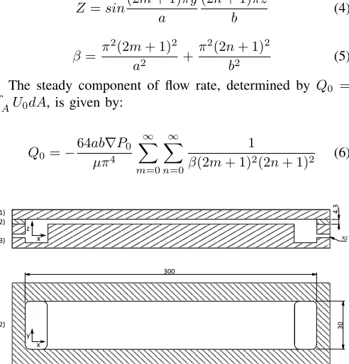
Fig. 1: Acrylic test piece containing rectangular channel 300
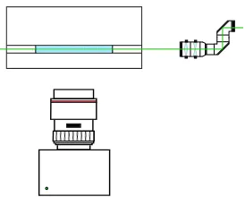
Fig. 2: Laser and camera orientation set up to capture the velocity profile across the channel width.
The pressure gradient terms are calculated using the ex-pression for the cross-sectional flow rate at the mid-height of the channel, which is derived by integrating the corresponding velocity profile U0(y, b/2)from 0 toa:
Qcs,0=−
32a∇P0 µπ3
∞
X
m=0 ∞
X
n=0
sin[(2n+ 1)π2]
β(2m+ 1)2(2n+ 1) (7) Qcs,0 is computed through integration of the experimental
velocity profiles using a trapezoidal integration technique. Equation 7 is then solved for∇P0. The first 100 terms of each of the infinite sums are used during numerical computation in Matlab software.
C. Solution for Oscillating Flow
The Green function method is used to solve the momentum equation following Fan and Chao [11]. The (1/ρ)∇P term in Equation 2 is replaced by an impulsive pressure gradient given by the Dirac delta function. The system is at rest at
t = 0 and the momentum equation reduces to dU/dt =
δ(t). Immediately after the impulse is applied, the velocity is U(y, z,0+) = R
0δ(t)dt = 1, → 0
+ and there is no
driving force acting on the flow. Hence, the governing equation becomes homogenous:
ν∇2U−dU
dt = 0 (8)
but with an inhomogeneous initial conditionU(y, z,0+) = 1.
The solution to Equation 8 is defined as the Green function for the system:
Gu(y, z, t) =
16
ρπ2 ∞
X
m=0 ∞
X
n=0
e−νβtZ
(2m+ 1)(2n+ 1) (9)
By convolving this with a sinusoidally oscillating pressure gradient f(t) = ∇Pt ·cos(ωt), the solution for the local
instantaneous velocity is attained:
U0(y, z, t) =
Z t
0
f(τ)Gu(y, z, t−τ)dτ (10)
U0(y, z, t) =−16∇Pt ρπ2
∞
X
m=0 ∞
X
n=0
Z
(2m+ 1)(2n+ 1)
·νβcos(ωt) +ωsin(ωt)−e −νβt
ν2β2+ω2
(11)
The oscillating component of the total flow rate is derived as in the steady flow case:
Q0=−64ab∇Pt ρπ4
∞
X
m=0 ∞
X
n=0
1
(2m+ 1)2(2n+ 1)2 ·νβcos(ωt) +ωsin(ωt)−e
−νβt
ν2β2+ω2
(12)
which is sinusoidal with normalized oscillation amplitude
Qt/Q0. The cross-sectional flow rate, used to calculate the
transient pressure gradient component ∇Pt, is derived as
before:
Qcs(z, t) =−
32a∇Pt µπ3
∞
X
m=0 ∞
X
n=0
sin[(2n+ 1)π2] (2m+ 1)2(2n+ 1) · νβcos(ωt) +ωsin(ωt)−e
−νβt
ν2β2+ω2
(13)
Starting from rest, these quantities will contain transients for a period after the motion starts governed by the e−νβt term
which tends to zero in the steady periodic state. For calculation of the pulsating values, the mean and oscillating components are simply summed, owing to the linearity of Equation 2.
III. EXPERIMENTAL
A. Apparatus
1) Channel Test Section: The test piece consists of a single rectangular channel 300 mm long × 30 mm wide × 4.2
0 0.005 0.01 0.015
0 2 4 6 8 10 12 14
y [m]
U [m/s]
[image:3.612.321.546.510.688.2]Re = 19 Re = 29 Re = 38 Re = 48 Re = 58 Re = 67 Re = 77 Re = 87
0 5 10 15 −2
0 2 4 6 8 10 12
(a)OPulsatingOProfiles
yO[mm]
UO[mm/s]
0 5 10 15
−5 −4 −3 −2 −1 0 1 2 3 4 5
(b)OOscillatingOProfiles
yO[mm]
UO[mm/s]
0 π/5
2π/5
3π/5
4π/5
π
6π/5
7π/5
8π/5
[image:4.612.94.523.57.280.2]9π/5
Fig. 4: Phase-averaged pulsating (non-zero mean) and oscillating (zero mean) velocity profiles for Womersley number W o
= 7.45 (f = 0.5 Hz), mean Reynolds number Re = 48, and flow rate oscillation amplitude Qt/Q0 = 0.75. Solid lines and
symbols represent analytical solutions and experimental measurements respectively.
mmhigh laser cut from optically transparent acrylic, covered above and below by similar acrylic pieces. The inlet and outlet are machined into the piece at the base of the channel as illustrated in Figure 1. Sealing is achieved using silicone rubber gaskets. The viewing window is 75mmlong centered in the 300 mm to reduce asymmetrical effects. To facilitate optical access through the narrow edinvage of the channel plate, the machined surfaces are polished.
2) Gear Pump Pulsator: The flow is driven by a micro an-nular gear pump (HNP Mikrosysteme mzr-4605, 72mL/min) and operated using a Terminal Box S-G05 controller and Matlab software. Pulsating flow of a given mean, frequency and amplitude is generated by discretising the corresponding sinusoid into a finite number of time steps. At each interval, a timer function executes and writes a motor speed to the controller based on the phase of the period. A maximum step size of 0.5 s is used to ensure that the inertia of the motor causes a smooth temporal flow rate. A counter implemented in the timer function records the phase of the output flow. At desired phase values, a digital output pin on the motor controller is set to high and sent to the imaging system to trigger image capture.
3) Particle Image Velocimetry: The imaging system uses particle image velocimetry (PIV) to measure the behaviour of the flow. The flow is seeded with 4 µm diameter nylon-12 tracer particles (TSI P/N 10084) which are illuminated by a Quantel Twins Big Sky Laser system. A pair of individual lamp-pumped Nd:YAG, 200mJ per pulse lasers are combined in a single optical axis to produce collimated green light of 532nmwavelength. A laser plane of about 1mmthickness is achieved using concave and convex lenses (with focal lengths of 1000 mmand -25 mmrespectively) to focus and diverge the light. Images are captured by a TSI 4M P (2352 x 1768
pixel) PowerView CCD camera with a close-up Sigma DG 105 mm focal length macro lens, interfaced to the PC using an Xcelera frame grabber. The camera and laser system are set up at right angles to each other to capture the velocity distribution across the 30 mm channel width, as illustrated in Figure 2. System timing is controlled by a Model 610035 LaserPulse Synchroniser which automates signal generation to the laser flash lamps and Q-switches, the camera and the frame grabber with 1nstime resolution. This control unit also reads an external 800 µs TTL pulse trigger signal from the pump controller to phase-lock measurements to the sinusoidal oscillation of the flow. The entire PIV system is completely controlled by a dedicated computer running TSI’s Insight 4G data acquisition software.
B. Analysis
In order to validate the experimental setup, steady flows with Reynolds number 19–87 are circulated through the channel and compared to theory. The symbols of Figure 3 plot the experimentally measured velocity profiles near the mid-axial length. The analytical velocity profiles with matching cross-sectional flow rates, plotted by solid lines, are in agreement with experiment to within 15.9%.
The axial evolution of the measured velocity field is investi-gated to ensure that the flow is fully-developed in the viewing window of the channel. Velocity distributions are found to vary by a maximum of 16.7% from the mean, with the maximum discrepancy occurring near the wall of the channel y = 0.5
0 5 10 15 0
2 4 6 8 10 12
(a)cPulsatingcProfiles
yc[mm]
Uc[mm/s]
0 5 10 15
−6
−4
−2 0 2 4 6
(b)cOscillatingcProfiles
yc[mm]
Uc[mm/s]
0
π/5 2π/5 3π/5 4π/5
π
[image:5.612.96.519.57.280.2]6π/5 7π/5 8π/5 9π/5
Fig. 5: Phase-averaged pulsating (non-zero mean) and oscillating (zero mean) velocity profiles for Womersley number W o
= 2.36 (f = 0.05 Hz), mean Reynolds numberRe = 48, and flow rate oscillation amplitude Qt/Q0 = 0.75. Solid lines and
symbols represent analytical solutions and experimental measurements respectively.
technique in Matlab, are found to vary by less than 3.3% in the xdirection.
IV. RESULTS& DISCUSSION
In this section, experimental results for pulsating flows with mean Reynolds number Re = 48, flow rate oscillation amplitudeQt/Q0= 0.75 and Womersley numbersW o= 7.45
and 2.36 (f = 0.5 and 0.05Hz) are presented and compared to theoretical predictions using the analytical solution of Section II.
A. Velocity Profiles
The symbols of Figure 4(a) plot the experimentally mea-sured instantaneous velocity profiles of the high Womersley number pulsations W o = 7.45. The flow is characterized by steep near-wall velocity gradients and may be approximated as a slug. Furthermore, significant flow reversal occurs at the minimum of the pulsation cycle. The transient components of velocity are computed through subtraction of the mean steady profile Re = 48 from the pulsating profiles. Plotted by the symbols of Figure 4(b), these instantaneous oscillating veloc-ity distributions reveal the presence of a near-wall velocveloc-ity overshoot. The local velocity magnitudes are large relative to the wall velocity of the steady profile and dictate the near-wall behaviour of the pulsating flow. For sufficiently large
Qt/Q0, local reversal occurs despite an invariably positive
flow rate. The main body of fluid lags that closer to the wall, indicating that the flow is dominated by inertia. Consequently, the main fluid body lags the accelerating pressure gradient by 1.35 radians according to the analytical solution. Near the wall however, viscous stresses reduce the momentum of fluid layers which are inclined to reverse quickly when the pressure
gradient reverses leading to the observed annular effects and inflexion points.
To determine the analytical profiles, a sine wave is fitted to the cross-sectional flow rates of the experimental measure-ments. Any deviation from the fitted sine wave is largely as a result of timing errors in the imaging system. Slight corrections are made to instantaneous phases to ensure that the flow rate of the analytical velocity profile matches that of experiment. The solid lines of Figure 4, plotting the analytical distributions, indicate that the local time-resolved behaviour of inertia-dominated pulsating flow is well captured by theory. Pulsating velocity profiles that are universally positive have a maximum deviation of16.6%, which occurs near the channel wall. The 20.2% maximum error of velocity profiles that experience flow reversal is calculated at locations 0.8 mm
further than the point of zero velocity, which introduces large percentage errors. The discrepancy reduces in the bulk of the fluid with the majority (y > 5mm) of all phase-averaged profiles within about 8% of theory. The oscillating velocity profiles typically have less absolute deviation from theory since some experimental error is removed upon subtraction of the mean from the pulsating profiles; however, the lower velocities result in relative errors of similar magnitude.
Figure 5(a) plots the pulsating velocity distributions for
wall. The theoretically estimated phase delay between the flow rate and pressure gradient of 0.6 radians confirms that the flow is in the transitional frequency regime. As before, the mathematical solutions capture the temporal behaviour of the flow accurately. The largest variation of 28%, occurring near the wall y = 0.5 mm, reduces to a maximum of 10.6% for
y >0.8 mm.
Flows that are approximately quasi-steady in nature require very high pulsation periods (T >50s) in such a large channel and have not been characterized in the current work due to time constraints. By definition, these barely transient flows are very similar to steady flows and are thus unlikely to measurably improve heat transfer compared to non-pulsating flows.
B. Anticipated Effects on Heat Transfer and Coefficient of Performance (COP)
A mechanism for heat transfer enhancement in pulsating flow has not been explicitly demonstrated in the literature. It seems intuitive that the elevated velocity gradients and narrow boundary layers of more quickly pulsating flows would lead to a simultaneous reduction in the thickness of the thermal boundary layer. Alternatively, pulsation may create more com-plex flow structures and mixing effects. The current work serves to investigate the plausibility of the former hypothesis with respect to fluid mechanical behaviour, by examining near-wall velocity gradients using ensemble-averaged mea-surements of the flow field. Scrutiny of the latter method is restricted since instantaneous structures in the flow may be concealed by phase-averaging.
The noted increase in magnitude of the wall shear rates in the high-frequency regime may induce a narrowing of the thermal boundary layer, a decrease in thermal resistance of the system and cause heat transfer enhancement. However, the reversal of flow for periods of the cycle would act to transport hot fluid towards the cooler entrance region and lessen the driving temperature differential between the channel wall and working fluid in heat transfer applications. Hence, the overall effect of steep velocity gradients and flow reversal on heat transfer remains unclear. Furthermore, inertial losses cause high pressure drops in the system and require a high work input. According to the analytical solution, the amplitude of the oscillating pressure gradient per unit flow rate is approx-imately 6.6 times that of steady flow. In the mid-frequency regime, the requisite energy input falls to 1.2 times that needed for steady flow as the inertial losses decrease; however, the near-wall slopes of the velocity profiles are not universally enhanced. While favorably steep gradients are observed as the flow accelerates, heat transfer may be degraded during deceleration when the slope levels out. The flow may hence demonstrate both higher and lower heat transfer during the cy-cle. A useful parameter for assessing the compromise between energy consumption and any heat transfer enhancement is the coefficient of performance (COP), which measures the ratio of heat removed to work input to the pump. To optimize the COP of a pulsating flow system, the hydrodynamic and thermal behaviour must be analyzed over a wide range of frequencies and amplitudes.
V. CONCLUSION
This work has measured the instantaneous velocity profiles of inertia-dominated and transitional pulsating flows in a single-phase channel flow using particle image velocimetry (PIV). The results are corroborated by the analytical solution for flow in a two-dimensional rectangular channel, solved using the Green functions method [11]. Conversely, the an-alytical solution for the local, time-resolved velocity profiles is preliminarily validated for the parameters tested.
A qualitative inspection of the near-wall velocity gradients was performed to ascertain the heat transfer enhancing poten-tial of the flows according to a frequently hypothesized mech-anism involving successive narrowing of the hydrodynamic and thermal boundary layers. For the dimensionless values of frequency W o = 7.45 and 2.36 and amplitude Qt/Q0 =
0.75 tested, the instantaneous velocity gradients at the wall are qualitatively observed to change with respect to those of steady flow. For W o = 7.45, higher values are consistently noted throughout the cycle. However, the effect of flow reversal in the vicinity of the wall is uncertain and requires further investigation. AtW o = 2.36, the wall shear rate is increased during acceleration and reduced while decelerating.
With respect to practical applications, this study under-lines the potential for heat transfer enhancement in pulsating flow. While it seems that the increased inertial losses may require larger work input, diaphragm micro pumps that are inherently pulsatile currently offer flow rates of 35 mL/min
using piezoelectric elements with low power consumption. The generic macro-scale channel geometry of this study thus acts as reference case for future mini- and microchannel cooling solutions using commercially-available technology.
ACKNOWLEDGMENT
The authors would like to acknowledge the financial support of the Irish Research Council (IRC) under grant number EPSPG/2013/618.
NOMENCLATURE
A cross-sectional area [m2] Dh channel hydraulic diameter [m] Gu Green function for velocity P pressure [P a]
Re steady Reynolds number (=U Dh/ν) Q0 steady flow rate component[m3/s]
Q0 transient flow rate component[m3/s]
Qcs,0 steady cross-sectional flow rate component[m2/s] Qcs,t oscillating cross-sectional flow rate amplitude[m2/s] Qt oscillating flow rate amplitude[m3/s]
T period of oscillation[s]
U0 steady velocity component[m/s] U0 transient velocity component[m/s]
Ut oscillating velocity amplitude [m/s] W o Womersley number (=12Dh
p
2πf /ν)
Z function defined as Equation 4
a, b channel width, height [m]
f oscillation frequency [Hz]
m, n summation indices
x axial flow coordinate[m]
y, z coordinates normal to flow direction [m]
Greek symbols
β function defined as Equation 5
δ Dirac delta function
µ viscosity [kg/ms]
ν kinematic viscosity [m2/s] ρ density [kg/m3]
ω angular oscillation frequency[rad/s]
Operators
∇ differential operator d/dx
∇2 Laplacian operator δ2/δy2+δ2/δz2
Subscripts
0 steady flow component
t oscillating flow amplitude
REFERENCES
[1] J. Brodkin, “Bandwidth explosion: As internet use soars, can bot-tlenecks be averted.” Arstechnica, May 1, 2012. [Online]. Avail-able: http://arstechnica.com/business/2012/05/bandwidth-explosion-as-internet-use-soars-can-bottlenecks-be-averted/. [Accessed: 2015-11-21]. [2] N. Jeffers, J. Stafford, K. Nolan, B. Donnelly, R. Enright, J. Punch, A. Waddell, L. Erlich, J. O’Connor, A. Sexton, R. Blythman, and D. Hernon, “Microfluidic cooling of photonic integrated circuits (PICs),” in Fourth European Conference on Microfluidics, Limerick, Ireland, 2014.
[3] S. Kandlikar, “Heat transfer mechanisms during flow boiling in mi-crochannels,” in ASME 2003 1st International Conference on Mi-crochannels and Minichannels, pp. 33–46, American Society of Me-chanical Engineers, 2003.
[4] T. Persoons, T. Saenen, T. Van Oevelen, and M. Baelmans, “Effect of flow pulsation on the heat transfer performance of a minichannel heat sink,”Journal of Heat Transfer, vol. 134, no. 9, p. 091702, 2012. [5] G. Stokes,On the effect of the internal friction of fluids on the motion
of pendulums, vol. 9. Pitt Press, 1851.
[6] J. Womersley, “Method for the calculation of velocity, rate of flow and viscous drag in arteries when the pressure gradient is known,” The Journal of physiology, vol. 127, no. 3, pp. 553–563, 1955.
[7] E. Richardson and E. Tyler, “The transverse velocity gradient near the mouths of pipes in which an alternating or continuous flow of air is established,”Proceedings of the Physical Society, vol. 42, no. 1, p. 1, 1929.
[8] T. Sexl, “ ¨Uber den von eg richardson entdeckten annulareffekt ,”
Zeitschrift f¨ur Physik, vol. 61, no. 5-6, pp. 349–362, 1930.
[9] S. Uchida, “The pulsating viscous flow superposed on the steady laminar motion of incompressible fluid in a circular pipe,”Zeitschrift f¨ur angewandte Mathematik und Physik ZAMP, vol. 7, no. 5, pp. 403– 422, 1956.
[10] H. Ito, “Theory of laminar flow through a pipe with non-steady pressure gradients,”Proceedings of the Institute of High Speed Mechanics, p. 163, 1953.
[11] C. Fan and B. Chao, “Unsteady, laminar, incompressible flow through rectangular ducts,”Zeitschrift f¨ur angewandte Mathematik und Physik ZAMP, vol. 16, no. 3, pp. 351–360, 1965.
[12] E. Denison, W. Stevenson, and R. Fox, “Pulsating laminar flow measure-ments with a directionally sensitive laser velocimeter,”AIChE Journal, vol. 17, no. 4, pp. 781–787, 1971.
[13] J. Harris, G. Peev, and W. Wilkinson, “Velocity profiles in laminar oscillatory flow in tubes,”Journal of Physics E: Scientific Instruments, vol. 2, no. 11, p. 913, 1969.
[14] T. Muto and K. Nakane, “Unsteady flow in circular tube: Velocity distribution of pulsating flow,” Bulletin of JSME, vol. 23, no. 186, pp. 1990–1996, 1980.
[15] D. Eckmann and J. Grotberg, “Experiments on transition to turbulence in oscillatory pipe flow,”Journal of Fluid Mechanics, vol. 222, pp. 329– 350, 1991.