Core Semantic First: A Top down Approach for AMR Parsing

(1)

Proceedings of the 2019 Conference on Empirical Methods in Natural Language Processing 3799

Core Semantic First: A Top-down Approach for AMR Parsing

∗

Deng Cai

The Chinese University of Hong Kong

[email protected]

Wai Lam

The Chinese University of Hong Kong

[email protected]

Abstract

We introduce a novel scheme for parsing a piece of text into its Abstract Meaning Repre-sentation (AMR): Graph Spanning based Pars-ing (GSP). One novel characteristic of GSP is that it constructs a parse graph incremen-tally in a top-down fashion. Starting from the root, at each step, a new node and its con-nections to existing nodes will be jointly pre-dicted. The output graph spans the nodes by the distance to the root, following the intuition of first grasping the main ideas then digging into more details. Thecore semantic first prin-ciple emphasizes capturing the main ideas of a sentence, which is of great interest. We evalu-ate our model on the levalu-atest AMR sembank and achieve the state-of-the-art performance in the sense that no heuristic graph re-categorization is adopted. More importantly, the experiments show that our parser is especially good at ob-taining the core semantics.

1 Introduction

Abstract Meaning Representation (AMR) ( Ba-narescu et al.,2013) is a semantic formalism that encodes the meaning of a sentence as a rooted la-beled directed graph. As illustrated by an example in Figure1, AMR abstracts away from the surface forms in text, where the root serves as a rudimen-tary representation of the overall focus while the details are elaborated as the depth of the graph in-creases. AMR has been proved useful for many downstream NLP tasks, including text summariza-tion (Liu et al., 2015;Hardy and Vlachos,2018) and question answering (Mitra and Baral,2016).

The task of AMR parsing is to map natural lan-guage strings to AMR semantic graphs automat-ically. Compared to constituent parsing (Zhang

∗_{The work described in this paper is substantially}

sup-ported by a grant from the Research Grant Council of the Hong Kong Special Administrative Region, China (Project Code: 14204418). The first author is grateful for the discus-sions with Zhisong Zhang and Zhijiang Guo.

strike-01

time sudden

earthquake

time manner

ARG2

prosper-01 happiness

op1 op2

big mod

[image:1.595.334.499.219.368.2]

such mod

Figure 1: AMR for the sentence “During a time of pros-perity and happiness, such a big earthquake suddenly struck.”, where the subgraphs close to the root repre-sent the core semantics.

and Clark,2009) and dependency parsing (K¨ubler et al., 2009), AMR parsing is considered more challenging due to the following characteristics: (1) The nodes in AMR have no explicit alignment to text tokens; (2) The graph structure is more complicated because of frequent reentrancies and non-projective arcs; (3) There is a large and sparse vocabulary of possible node types (concepts).

Many methods for AMR parsing have been de-veloped in the past years, which can be catego-rized into three main classes: Graph-based parsing (Flanigan et al.,2014;Lyu and Titov, 2018) uses a pipeline design for concept identification and re-lation prediction. Transition-based parsing (Wang et al.,2016;Damonte et al.,2017;Ballesteros and Al-Onaizan, 2017;Guo and Lu, 2018;Liu et al.,

2018;Wang and Xue,2017) processes a sentence from left-to-right and constructs the graph incre-mentally. The third class is seq2seq-based parsing (Barzdins and Gosko,2016;Konstas et al.,2017;

(2)

While existing graph-based models cannot suf-ficiently model the interactions between individual decisions, the autoregressive nature of transition-based and seq2seq-transition-based models makes them suf-fer from error propagation, where later decisions can easily go awry, especially given the complex-ity of AMR. Since capturing the core semantics of a sentence is arguably more important and useful in practice, it is desirable for a parser to have a global view and a priority for capturing the main ideas first. In fact, AMR graphs are organized in a hierarchy that the core semantics stay closely to the root, for which a top-down parsing scheme can fulfill the desiderata. For example, in Figure 1, the subgraph in the red box already conveys the core meaning “an earthquake suddenly struck at a particular time”, and the subgraph in the blue box further informs that “the earthquake was big” and “the time was of prosperity and happiness”.

We propose a novel framework for AMR pars-ing known as Graph Spannpars-ing based Parspars-ing (GSP). One novel characteristic of GSP is that, to our knowledge, it is the first top-down AMR parser.1 _{GSP performs parsing in an}

incremen-tal, root-to-leaf fashion, but still maintains a global view of the sentence and the previously derived graph. At each step, it generates the connecting arcs between the existing nodes and the coming new node, upon which the type of the new node (concept) is jointly decided. The output graph spans the nodes by the distance to the root, fol-lowing the intuition of first grasping the main ideas then digging into more details. Compared to pre-vious graph-based methods, our model is capa-ble of capturing more complicated intra-graph in-teractions, while reducing the number of parsing steps to be linear in the sentence length.2

Com-pared to transition-based methods, our model re-moves the left-to-right restriction and avoids so-phisticated oracle design for handling the com-plexity of AMR graphs.

Notably, most existing methods including the state-the-of-art parsers often rely on heavy graph re-categorization for reducing the complexity of the original AMR graphs. For graph re-categorization, specific subgraphs of AMR are grouped together and assigned to a single node with a new compound category (Werling et al.,

1_{Depth-first traversal in seq2seq models does not produce}

a strictly top-down order due to the reentrancies in AMR.

2_{Since the size of AMR graph is approximately linear in}

the length of sentence.

2015;Wang and Xue, 2017; Foland and Martin,

2017; Lyu and Titov, 2018; Groschwitz et al.,

2018;Guo and Lu,2018). The hand-crafted rules for re-categorization are often non-trivial, requir-ing exhaustive screenrequir-ing and expert-level man-ual efforts. For instance, in the re-categorization system of Lyu and Titov (2018), the graph fragment “temporal-quantity :ARG_−→3−of rate-entity-91 :−→unit year :quant−→ 1”

will be replaced by one single nested node

“rate-entity-3(annual-01)”. There are

hundreds of such manual heuristic rules. This kind of re-categorization has been shown to have con-siderable effects on the performance (Wang and Xue,2017;Guo and Lu,2018). However, one is-sue is that the precise set of re-categorization rules differs among different models, making it difficult to distinguish the performance improvement from model optimization or carefully designed rules. In fact, some work will become totally infeasible when removing this re-categorization step. For ex-ample, the parser ofLyu and Titov(2018) requires tight integration with this step as it is built on the assumption that an injective alignment exists be-tween sentence tokens and graph nodes.

We evaluate our parser on the latest AMR sem-bank and achieve competitive results to the state-of-the-art models. The result is remarkable since our parser directly operates on the original AMR graphs and requires no manual efforts for graph re-categorization. The contributions of our work are summarized as follows:

• We propose a new method for learning AMR parsing that produces high-quality core se-mantics.

• Without the help of heuristic graph re-categorization which requires expensive expert-level manual efforts for designing re-categorization rules, our method achieves state-of-the-art performance.

2 Related Work

Currently, most AMR parsers can be catego-rized into three classes: (1) Graph-based meth-ods (Flanigan et al., 2014, 2016; Werling et al.,

2015; Foland and Martin, 2017; Lyu and Titov,

(3)

max-imum spanning connected subgraph algorithm to select the final graph. The major deficiency is that the concept identification and relation prediction are strictly performed in order, yet the interactions between them should benefit both sides (Zhou et al., 2016). In addition, for computational effi-cacy, usually only first-order information is con-sidered for edge scoring. (2) Transition-based methods (Wang et al.,2016;Damonte et al.,2017;

Wang and Xue,2017;Ballesteros and Al-Onaizan,

2017; Liu et al., 2018; Peng et al., 2018; Guo and Lu,2018;Naseem et al.,2019) borrow tech-niques from shift-reduce dependency parsing. Yet the non-trivial nature of AMR graphs (e.g., reen-trancies and non-projective arcs) makes the tran-sition system even more complicated and difficult to train (Guo and Lu, 2018). (3) Seq2seq-based methods (Barzdins and Gosko,2016;Peng et al.,

2017; Konstas et al., 2017; van Noord and Bos,

2017) treat AMR parsing as sequence-to-sequence problem by linearizing AMR graphs, thus exist-ing seq2seq models (Bahdanau et al.,2014;Luong et al., 2015) can be readily utilized. Despite its simplicity, the performance of the current seq2seq models lag behind when the training data is lim-ited. The first reason is that seq2seq models are often not as effective on smaller datasets. The sec-ond reason is that the linearized AMRs add the challenges of making use of the graph structure information.

There are also some notable exceptions. Peng et al. (2015) introduce a synchronous hyperedge replacement grammar solution. Pust et al.(2015) regard the task as a machine translation problem, while Artzi et al.(2015) adapt combinatory cate-gorical grammar.Groschwitz et al.(2018); Linde-mann et al.(2019) view AMR graphs as the struc-ture AM algebra.

Most AMR parsers require an explicit align-ment between tokens in the sentences and nodes in the AMR graph during training. Since such in-formation is not annotated, a pre-trained aligner (Flanigan et al.,2014;Pourdamghani et al.,2014;

Liu et al.,2018) is often required. More recently,

Lyu and Titov (2018) demonstrate that the align-ments can be treated as latent variables in a joint probabilistic model.

3 Background and Overview

3.1 Background of Multi-head Attention

The multi-head attention mechanism introduced byVaswani et al.(2017) is used as a basic building block in our framework. The multi-head attention consists ofH attention heads, and each of which

learns a distinct attention function. Given a query vectorx and a set of vectors{y1, y2, . . . , ym} or

in shorty1:m, for each attention head, we project

xandy1:minto distinct query, key, and value

rep-resentationsq _∈ _Rd_,_K _∈_Rm×d_and_V _∈_Rm×d

respectively, wheredis the dimension of the

vec-tor space. Then we perform scaled dot-product at-tention (Vaswani et al.,2017):

a=softmax(Kq√ )

d

attn=aV

wherea _∈ Rm _{is the attention vector (a}

distribu-tion over all inputy1:m) andattnis the weighted

sum of the value vectors. Finally, the outputs of all attention heads are concatenated and projected to the original dimension ofx. For brevity, we will

denote the whole attention procedure described above as a functionT(x, y1:m).

Based on the multi-head attention, the Trans-former encoder (Vaswani et al., 2017) uses self-attention for context information aggregation when given a set of vectors (e.g., word embed-dings in a sentence or node embedembed-dings in a graph).

3.2 Overview

Figure2 depicts the major neural components in our proposed framework: The Sentence Encoder component and the Graph Encoder component are designed for token-level sentence representation and node-level graph representation respectively. Given an input sentencew = (w1, w2, . . . , wn),

wherenis the sentence length, the Sentence

En-coder component will first read the whole sentence and encode each wordwi into the hidden statesi.

The initial graphG0is always initialized with one

dummy node d∗ and a previously generated

con-ceptcj is encoded into the hidden statevj by the

Graph Encoder component.

At each time step t, the Focus Selection

com-ponent reads both the sentence representations1:n

and the graph representation v0:t−1 of Gt−1

(4)

w₁ w₂ wn

s₁ s₂ sn

c₁ c₂ c3

v₁ v₂ v₃

Focus Selection

…

ht _{_agi

t }ki= 1

as t

Gt−1

Sentence Encoder Graph Encoder

×k parser state 1 2 3 4 5

Concept Prediction Relation Classification Relation Identification

? ct

d*

Figure 5: A single layer of the Recursive Neural Ten-sor Network. Each dashed box represents one ofd-many slices and can capture a type of influence a child can have on its parent.

The RNTN uses this definition for computingp1:

p1=f 

b c T

V[1:d] 

b c +W



b c

!

,

whereWis as defined in the previous models. The next parent vectorp2in the tri-gram will be

com-puted with the same weights:

p2=f 

a p1

T V[1:d]



a p1 +W



a p1 !

.

The main advantage over the previous RNN model, which is a special case of the RNTN when Vis set to0, is that the tensor can directly relate in-put vectors. Intuitively, we can interpret each slice of the tensor as capturing a specific type of compo-sition.

An alternative to RNTNs would be to make the compositional function more powerful by adding a second neural network layer. However, initial exper-iments showed that it is hard to optimize this model and vector interactions are still more implicit than in the RNTN.

4.4 Tensor Backprop through Structure We describe in this section how to train the RNTN model. As mentioned above, each node has a

softmaxclassifier trained on its vector representa-tion to predict a given ground truth or target vector t. We assume the target distribution vector at each node has a 0-1 encoding. If there areCclasses, then it has lengthCand a 1 at the correct label. All other entries are 0.

We want to maximize the probability of the cor-rect prediction, or minimize the cross-entropy error between the predicted distributionyi₂_RC⇥1_at

nodeiand the target distributionti₂_RC⇥1_{at that}

node. This is equivalent (up to a constant) to mini-mizing the KL-divergence between the two distribu-tions. The error as a function of the RNTN parame-ters✓= (V, W, Ws, L)for a sentence is:

E(✓) =X

i

X

j ti

jlogyij+ k✓k2 (2)

The derivative for the weights of thesoftmax clas-sifier are standard and simply sum up from each node’s error. We definexi_{to be the vector at node} i(in the example trigram, thexi ₂ _Rd⇥1_{’s are} (a, b, c, p1, p2)). We skip the standard derivative for Ws. Each node backpropagates its error through to the recursively used weightsV, W. Let i,s₂_Rd⇥1

be thesoftmaxerror vector at nodei: i,s₌ _WT

s(yi ti) ⌦f0(xi), where⌦is the Hadamard product between the two vectors andf0_{is the element-wise derivative of}f which in the standard case of usingf= tanhcan be computed using onlyf(xi₎_.

The remaining derivatives can only be computed in a top-down fashion from the top node through the tree and into the leaf nodes. The full derivative for VandWis the sum of the derivatives at each of the nodes. We define the complete incoming error messages for a nodeias i,com_{. The top node, in} our casep2, only received errors from the top node’s softmax. Hence, p2,com₌ p2,s_{which we can} use to obtain the standard backprop derivative for W(Goller and K¨uchler, 1996; Socher et al., 2010). For the derivative of each slicek= 1, . . . , d, we get:

@Ep2

@V[k]=

p2,com k  a p1  a p1 T ,

where p2,com

k is just thek’th element of this vector. Now, we can compute the error message for the two Figure 5: A single layer of the Recursive Neural

Ten-sor Network. Each dashed box represents one ofd-many slices and can capture a type of influence a child can have on its parent.

p1=f



b c T

V[1:d]b c +W

_b

c

!

,

whereWis as defined in the previous models. The next parent vectorp2in the tri-gram will be com-puted with the same weights:

p2=f



a p1

T V[1:d]a

p1 +W

_a

p1

!

.

The main advantage over the previous RNN model, which is a special case of the RNTN when

Vis set to0, is that the tensor can directly relate in-put vectors. Intuitively, we can interpret each slice of the tensor as capturing a specific type of compo-sition.

4.4 Tensor Backprop through Structure

We describe in this section how to train the RNTN model. As mentioned above, each node has a

softmaxclassifier trained on its vector representa-tion to predict a given ground truth or target vector

t. We assume the target distribution vector at each node has a 0-1 encoding. If there areCclasses, then it has lengthCand a 1 at the correct label. All other entries are 0.

We want to maximize the probability of the cor-rect prediction, or minimize the cross-entropy error between the predicted distributionyi ₂ _RC⇥1_at nodeiand the target distributionti₂_RC⇥1_{at that} node. This is equivalent (up to a constant) to mini-mizing the KL-divergence between the two distribu-tions. The error as a function of the RNTN parame-ters✓= (V, W, Ws, L)for a sentence is:

E(✓) =X

i

X

j ti

jlogyij+ k✓k2 (2)

The derivative for the weights of thesoftmax clas-sifier are standard and simply sum up from each node’s error. We definexi_{to be the vector at node} i(in the example trigram, thexi ₂ _Rd⇥1_{’s are} (a, b, c, p1, p2)). We skip the standard derivative for Ws. Each node backpropagates its error through to the recursively used weightsV, W. Let i,s₂_Rd⇥1 be thesoftmaxerror vector at nodei:

i,s₌ _WT

s(yi ti) ⌦f0(xi),

where⌦is the Hadamard product between the two vectors andf0_{is the element-wise derivative of}_f which in the standard case of usingf= tanhcan be computed using onlyf(xi₎_.

The remaining derivatives can only be computed in a top-down fashion from the top node through the tree and into the leaf nodes. The full derivative for

V andWis the sum of the derivatives at each of the nodes. We define the complete incoming error messages for a nodeias i,com_{. The top node, in}

our casep2, only received errors from the top node’s softmax. Hence, p2,com₌ p2,s_{which we can}

use to obtain the standard backprop derivative for

W(Goller and K¨uchler, 1996; Socher et al., 2010). For the derivative of each slicek= 1, . . . , d, we get:

@Ep2

@V[k]= p2,com k  a p1  a p1 T ,

where p2,com

k is just thek’th element of this vector.

Now, we can compute the error message for the two f

p1=f



b c

T

V[1:d]b

c +W



b c

!

,

p2=f



a p1

T

V[1:d]a

p1 +W



a p1

!

.

We want to maximize the probability of the cor-rect prediction, or minimize the cross-entropy error between the predicted distributionyi₂_RC⇥1_at nodeiand the target distributionti₂_RC⇥1_{at that} node. This is equivalent (up to a constant) to mini-mizing the KL-divergence between the two distribu-tions. The error as a function of the RNTN parame-ters✓= (V, W, Ws, L)for a sentence is:

E(✓) =X

i X

j

ti

jlogyji+ k✓k2 (2)

The derivative for the weights of thesoftmax clas-sifier are standard and simply sum up from each node’s error. We definexi_{to be the vector at node}

i(in the example trigram, thexi

2 Rd⇥1_{’s are}

(a, b, c, p1, p2)). We skip the standard derivative for

Ws. Each node backpropagates its error through to

the recursively used weightsV, W. Let i,s₂_Rd⇥1 be thesoftmaxerror vector at nodei:

i,s₌ _WT

s(yi ti) ⌦f0(xi),

where⌦is the Hadamard product between the two vectors andf0_{is the element-wise derivative of}_f

which in the standard case of usingf= tanhcan be computed using onlyf(xi₎_.

VandWis the sum of the derivatives at each of the nodes. We define the complete incoming error messages for a nodeias i,com_{. The top node, in}

our casep2, only received errors from the top node’s

softmax. Hence, p2,com ₌ p2,s_{which we can}

@Ep2 @V[k]=

p2,com k _a p1 _a p1 T ,

where p2,com

Now, we can compute the error message for the two f +

p1=f



b c

T

V[1:d]b

c +W

_b

c

!

,

p2=f



a p1

T

V[1:d]a

p1 +W



a p1

!

.

We want to maximize the probability of the cor-rect prediction, or minimize the cross-entropy error between the predicted distributionyi ₂_RC⇥1_at nodeiand the target distributionti₂_RC⇥1_{at that} node. This is equivalent (up to a constant) to mini-mizing the KL-divergence between the two distribu-tions. The error as a function of the RNTN parame-ters✓= (V, W, Ws, L)for a sentence is:

E(✓) =X

i X

j

ti

jlogyij+ k✓k2 (2)

The derivative for the weights of thesoftmax clas-sifier are standard and simply sum up from each node’s error. We definexi_{to be the vector at node}

i(in the example trigram, thexi ₂ _Rd⇥1_{’s are}

(a, b, c, p1, p2)). We skip the standard derivative for

Ws. Each node backpropagates its error through to

the recursively used weightsV, W. Let i,s₂_Rd⇥1 be thesoftmaxerror vector at nodei:

i,s₌ _WT

s(yi ti)⌦f0(xi),

where⌦is the Hadamard product between the two vectors andf0_{is the element-wise derivative of}f

which in the standard case of usingf= tanhcan be computed using onlyf(xi₎_.

VandWis the sum of the derivatives at each of the nodes. We define the complete incoming error messages for a nodeias i,com_{. The top node, in}

our casep2, only received errors from the top node’s

softmax. Hence, p2,com₌ p2,s_{which we can}

@Ep2 @V[k]=

p2,com k  a p1  a p1 T ,

where p2,com

Now, we can compute the error message for the two

[image:4.595.120.483.64.292.2]

ct d* d* ? d* Gt

Figure 2: Model architecture of GSP, together with the decoding procedure at the time stept, where the read and write operations around the parser statehtfollow the order 1 → →2 →3 →4 5.

parser state carries the most useful information and serves as a writable memory during the expan-sion step. Next, the Relation Identification com-ponent decides which specific head nodes to ex-pand by computing the multiple attention scores

{agi

t }ki=1 over the existing nodes. New arcs are

generated according to the attention scores. Then the Concept Prediction component updates the parser statehtwith arc information, computes the

attention vectoras_t over the sentence and

accord-ingly chooses a specific part to generate the new concept ct. Finally, the Relation Classification

component is used to predict the relation labels be-tween the newly generated concept and its prede-cessors. Consequently an updated graphGtis

pro-duced andGtwill be processed for the next time

step. The whole decoding procedure is terminated if the newly generated concept is the special stop concept.

Our method expands the graph in a root-to-leaf fashion, nodes with shorter distances to the root will be introduced first. It follows a similar way that humans grasp the meaning: first seek-ing the main concepts then proceedseek-ing to the sub-structures governed by certain head concepts ( Ba-narescu et al.,2013).

During training, we use breadth-first search to decide the order of nodes. However, for nodes with multiple children, there still exist multiple valid selections. In order to define a deterministic

decoding process, we sort sibling nodes by their relations to the head node. We will present more discussions on the choice of sibling order in§5.3.

4 Framework Description

4.1 Sentence & Graph Representation

Transformer encoder architecture is employed for both the Sentence Encoder and the Graph encoder components. For sentence encoding, a special to-ken () is prepended to the input word sequence, whose final hidden states0 is regarded as an

ag-gregated summary of the whole sentence and used as the initial state in parsing steps.

The Graph Encoder component takes previously generated concept sequence

(c0, c1, . . . , ct−1) (c0 is the dummy node d∗)

as input. For computation efficiency and reducing error propagation, instead of encoding the edge information explicitly, we use the Transformer encoder to capture the interactions between nodes. Finally, the encoder outputs a sequence of node representations(v0, v1, . . . , vt−1).

4.2 Focus Selection

At each time step t, the Focus Selection

(5)

the following recurrence is applied byLtimes:

xl_t,+1₁ =LN(hl_t+T₁l+1(hl_t, s1:n))

x_t,l+1₂ =LN(xl_t,+1₁ +T₂l+1(xl_t,+1₁ , v0:t−1))

hl_t+1= max(xl_t,+1₂ W₁l+1+bl₁+1)W₂l+1+bl₂+1

whereT(·,·)is the multi-head attention function.

LN is the layer normalization (Ba et al.,2016) and

h0

t is always initialized with s0. For clarity, we

denote the last hidden statehL_t asht, as the parser

state at the time stept. We now proceed to present

the details of each decision stage of one parsing step, which is also illustrated in Figure2.

4.3 Relation Identification

Our Relation Identification component is inspired by a recent attempt of exposing auxiliary super-vision on attention mechanism (Strubell et al.,

2018). It can be considered as another attention layer over the existing graph, yet the attention weights explicitly indicate the likelihood of the new node being attached to a specific node. In other words, its aim is to answer the question of where to expand. Since a node can be attached to multiple nodes by playing different semantic roles, we utilize multi-head attention and take the maxi-mum over different heads as the final arc probabil-ities.

Formally, through a multi-head attention mech-anism takinght andv0:t−1 as input, we obtain a

set of attention weights {agi

t }ki=1, where k is the

number of attention heads andagi

t is thei-th

prob-ability vector. The probprob-ability of the arc between the new node and the node vj is then computed

byag_t,j = maxi(ag_t,ji). Intuitively, each head is in

charge of a set of possible relations (though not ex-plicitly specified). If certain relations do not exist between the new node and any existing node, the probability mass will be assigned to the dummy noded∗. The maximum pooling reflects that the

arc should be built once one relation is activated.3

The attention mechanism passes the arc deci-sions to later layers by the update of the parser state as follows:

ht=LN(ht+Warc

t−1

X

j=0 ag_t,jvj)

3_{We also found that there may exist more than one relation}

between two distinct nodes, however, it rarely happens.

4.4 Concept Prediction

Our Concept Prediction component uses a soft alignment between words and the new concept. Concretely, a single-head attentionas

tis computed

based on the parser statehtand the sentence

rep-resentation s1:n, whereast,i denotes the attention

weight of the word wi in the current time step.

This component then updates the parser state with the alignment information via the following equa-tion:

ht=LN(ht+Wconc

n

X

i=1 as_t,isi)

The probability of generating a specific con-ceptcfrom the concept vocabularyVis calculated asgen(c_|ht) = exp(xcTht)/Pc0_∈Vexp(x_c0Th_t),

where xc (forc ∈ V) denotes the model

param-eters. To address the data sparsity issue in con-cept prediction, we introduce a copy mechanism in similar spirit toGu et al.(2016). Besides gener-ation, our model can either directly copy an input tokenwi (e.g, for entity names) or mapwito one

conceptm(wi) according to the alignment

statis-tics4_{in the training data (e.g., for “went”, it would}

proposego). Formally, the prediction probability of a conceptcis given by:

P(c_|ht) =P(copy|ht)

n

X

i=1

as_t,i[[wi=c]]

+P(map_|ht) n

X

i=1

as_t,i[[m(wi) =c]]

+P(gen_|ht)gen(c|ht)

where[[. . .]]is the indicator function.P(copy|ht),

P(map|ht)andP(gen|ht)are the probabilities of

three prediction modes respectively, computed by a single layer neural network with softmax activa-tion.

4.5 Relation Classification

Lastly, the Relation Classification component em-ploys a multi-class classifier for labeling the arcs detected in the Relation Identification component. The classifier uses a biaffine function to score each label, given the head concept representationviand

the child vectorhtas input:

ei_t=hT_tW vi+UTht+VTvi+b

4_{Based on the alignments provided by}_{Liu et al.}₍₂₀₁₈_),

(6)

where W, U, V, b are model parameters. As sug-gested byDozat and Manning(2016), we project

vi and ht to a lower dimension for reducing the

computation cost and avoiding the overfitting of the model. The label probabilities are computed by a softmax function over all label scores.

4.6 Reentrancies

AMR reentrancy is employed when a node partici-pates in multiple semantic relations (with multiple parent nodes), and that is why AMRs are graphs, rather than trees. The reentrancies are often hard to treat. While previous work often either remove them (Guo and Lu, 2018) or relies on rule-based restoration in the postprocessing stage (Lyu and Titov,2018;van Noord and Bos,2017), our model provides a new and principled way to deal with reentrancies. In our approach, when a new node is generated, all its connections to already existing nodes are determined by the multi-head attention. For example, for a node withkparent nodes,k

dif-ferent heads will point to the those parent nodes respectively. For a better understanding of our model, a pseudocode is presented in Algorithm1.

4.7 Training and Inference

Our model is trained to maximize the log likeli-hood of the gold AMR graphs given sentences, i.e.

logP(G|w), which can be factorized as:

logP(G_|w) = m

X

t=1

logP(ct|Gt−1,w)

+ X

i∈pred(t)

logP(arcit|Gt−1,w)

+ X

i∈pred(t)

logP(relarcit|Gt−1,w)

wherem is the total number of vertices. The set of predecessor nodes ofct is denoted aspred(t).

arcit denotes the arc between ci and ct, and

relarcit indicates the arc label (relation type). As mentioned, GSP is an autoregressive model, such as seq2seq models and transition models, but it factors the distribution according to a top-down graph structure rather than a depth-first traversal or a left-to-right chain. Meanwhile, GSP has a clear separation of node, arc and relation label prob-abilities, interacting in a more interpretable and tighten manner.

Algorithm 1Graph Spanning based Parsing

Input: the input sentencew= (w1, w2, . . . , wn)

Output: the AMR graphGcorresponds tow. 3Learning Sentence Representation 1: w=(w0 =) + (w1, w2, . . . , wn)

2: s0, s1, s2, . . . , sn=Transformer(w)

3Initialization

3: initialize the graphG0 (c0 =d∗)

4: initialize time stept= 1

3Entering Main Spanning Loop 5: whileTruedo

6: h0, . . . , vt−1 = Transformer(c0:t−1)

7: ht= Focus Selection(s0, v0:t−1, s1:n)

8: ht= Relation Identification(ht, v0:t−1)

8: decide the parents nodespred(t)of ct

9: ht= Concept Prediction(ht, s1:n)

9: decide the node type of ct

10: ifct== then

11: break

12: end if

13: for i_∈pred(t)do

14: Relation Classification(ht, vi)

14: decide the edge type betweenctandci

15: end for

16: updateGt−1toGt

17: end while 18: return Gt−1

At the operational or testing time, the pre-diction for the input w is obtained via Gˆ =

arg maxG0P(G0|w). Rather than iterating over

all possible graphs, we adopt a beam search to approximate the best graph. Specifically, for each partially constructed graph, we only consider the top-K concepts obtaining the best single-step

probability (a product of the corresponding con-cept, arc, and relation label probability), whereK

is the beam size. Only the bestK graphs at each

time step are kept for the next expansion.

5 Experiments

5.1 Setup

We focus on the most recent LDC2017T10 dataset, as it is the largest AMR corpus. It consists of 36521, 1368, and 1371 sentences in the train-ing, development, and testing sets respectively.

We use Stanford CoreNLP (Manning et al.,

(7)

consists of the randomly initialized lemma, part-of-speech tag, and named-entity tag embeddings, as well as the output from a learnable CNN with character embeddings as inputs. The graph en-coder uses randomly initialized concept embed-dings and another char-level CNN. Model hyper-parameters are chosen by experiments on the de-velopment set. The details of the hyper-parameter settings are provided in the Appendix. During testing, we use a beam size of 8 for generating

graphs.5

Conventionally, the quality of AMR parsing results is evaluated using the Smatch tool (Cai and Knight,2013), which seeks for the maximum number of overlaps between two AMR annota-tions after decomposing AMR graphs into triples. However, the ordinary Smatch metric treats all triples equally regardless of their roles in the com-position of the whole sentence meaning. We refine the ordinary Smatch metric to take into considera-tion the noconsidera-tion of core semantics. Specifically, we compute:

• Smatch-weighted: This metric weights dif-ferent triples by their importance of compos-ing the core ideas. The root distancedof a

triple is defined as the minimum root distance of its involving nodes, the weight of the triple is then computed as:

w= min(₋d+dthr,1)

In other words, the weight has a linear decay in root distance untildthr. If two triples are

matched, the minimum importance score of them is obtained. In our experiments,dthris

set to 5.

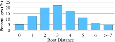
• Smatch-core: This metric only compares the subgraphs representing the main meaning. Precisely, we cut down AMR graphs by set-ting a maximum root distancedmaxand only

keep the nodes and edges within the thresh-old. dmax is set to4 in our experiments, of

which the remaining subgraphs still have a broad coverage of the original meaning, as il-lustrated by the distribution of root distance in Figure3.

Besides, we also evaluate the quality by comput-ing the followcomput-ing metrics.

5_{Our code can be found at}_{https://github.com/}

jcyk/AMR-parser.

0 5 10 15 20 25

0 1 2 3 4 5 6 >=7

Root Distance

P

erc

ent

age

[image:7.595.316.518.62.136.2]

s (%)

Figure 3: The distribution of root distance of concepts in the test set.

• complete-match (CM): This metric counts the number of parsing results that are com-pletely correct.

• root-accuracy (RA): This metric measures

the accuracy of the root concept identifica-tion.

5.2 Main Results and Case Study

The main result is presented in Table1. We com-pare our method with the best-performing models in each category as discussed in§2.

Concretely, van Noord and Bos (2017) is a character-level seq2seq model that achieves very competitive result. However, their model is very data demanding as it requires to train on addi-tional 100K sentence-AMR pairs generated by other parsers. Guo and Lu (2018) is a transition-based parser with refined search space for AMR. Certain concepts and relations (e.g., reentrancies) are removed to reduce the burdens during training.

Lyu and Titov(2018) is a graph-based method that achieves the best-reported result evaluated by the ordinary Smatch metric. Their parser uses differ-ent LSTMs for concept prediction, relation iddiffer-enti- identi-fication, and root identification sequentially. Also, the relation identification stage has the time com-plexity ofO(m2_log_m₎_where_m_{is the number of}

concepts. Groschwitz et al. (2018) views AMR as terms of the AM algebra (Groschwitz et al.,

2017), which allows standard tree-based parsing techniques to be applicable. The complexity of their projective decoder is O(m5). Last but not

least, all these models except for that ofvan No-ord and Bos(2017) require hand-crafted heuristics for graph re-categorization.

(8)

Model _{Re-ca. weighted core ordinary}Graph Smatch(%) RA(%) CM(%)

Buys and Blunsom(2017) No - - 61.9 -

-van Noord and Bos(2017) + 100K No 68.8 67.6 71.0 75.8 10.2

Guo and Lu(2018) Yes 63.5 62.3 69.8 63.6 9.4

Lyu and Titov(2018) Yes 66.6 67.1 74.4 59.1 10.2

Groschwitz et al.(2018) Yes - - 71.0 -

[image:8.595.84.514.62.174.2]

-Ours No 71.3 70.2 73.2 76.9 11.6

Table 1: Comparison with state-of-the-art methods (results on the test set). Results relying on heuristic rules for graph re-categorization are marked “Yes” in the Graph Re-ca. column.

generate-01

demand-01

travel-01

and

solve-01 pattern balance-01

function-01

settle-02

human

and

capacity

system transport use-01

land between

ARG1 ARG0

ARG1

ARG1-of

ARG2-of op1 op2

mod

ARG1

op1-of mod mod ARG1 op1 op2

ARG1

The solution is functional human patterns and a balance between transport system capacity and land use generated travel demand.

Input:

capacity

demand-01

system

travel-01 use-01 between

land solve-01

and

balance-01 op1 op2

pattern

settle-02

human

functional mod mod

ARG1

ARG1 ARG1

op1

mod ARG1

mod

op2 ARG1 ARG2

transport-01

Ours: Gold: L’18:

ARG1

capacity demand-01

system

transport-01

travel-01

use-01

land solve-01

and

balance-01 op1 op2

settle-03

human

function-01

mod ARG1-ofARG1 ARG2

poss

ARG1 purpose

ARG1 ARG2

generate-01 ARG0 ARG1-of pattern

Figure 4: Case study.

method in capturing the core ideas. Besides, our model achieves the highest root-accuracy (RA) and complete-match (CM), which further confirms the usefulness of a global view and the core se-mantic first principle.

Even evaluated by the ordinary Smatch met-ric, our model yields better results than all previ-ously reported models with the exception of Lyu and Titov (2018), which relies on a tremendous amount of manual heuristics for designing rules for graph re-categorization and adopts a pipeline approach. Note that our parser constructs the AMR graph in an end-to-end fashion with a bet-ter (quadratic) time complexity.

We present a case study in Figure4 with com-parison to the output of Lyu and Titov (2018)’s parser. As seen, both parsers make some mis-takes. Specifically, our method fails to iden-tify the concept generated-01. While Lyu and Titov (2018)’s parser successfully identifies it, their parser mistakenly treats it as the root of the whole AMR. It leads to a serious draw-back of making the sentence meaning be inter-preted in a wrong way. In contrast, our method shows a strong capacity in capturing the main idea “the solution is about some patterns and a bal-ance”. However, on the ordinary Smatch

met-S

m

at

ch-c

ore

0.55 0.61 0.68 0.74 0.80

Maximum Root Distance

0 1 2 3 4 5 6 full

Ours L’18 GL’18 vN’17

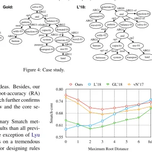
Figure 5: Smatch scores with different root distances. vN’17 isvan Noord and Bos(2017)’s parser with 100K additional training pairs. GL’18 isGuo and Lu(2018)’s parser. L’18 isLyu and Titov(2018)’s parser.

ric, their graph obtains a higher score (68% vs. 66%), which indicates that the ordinary Smatch is not a proper metric for evaluating the qual-ity of capturing core semantics. If we adopt the Smatch-weighted metric, our method achieves a better score i.e. 74% vs. 61%.

5.3 More Results

[image:8.595.209.519.226.534.2]

(9)

the maximum root distancedmax, compared with

several strong baselines and the state-of-the-art model. It demonstrates that our method is better at abstracting the core ideas of a sentence.

As discussed in § 3, there could be multiple

valid generation orders for sibling nodes in an AMR graph. We experiment with the following traversal variants: (1)random, which sorts the sib-ling nodes in completely random order. (2) rela-tion freq., which sorts the sibling nodes accord-ing to their relations to the head node. We assign higher priorities to relations that occur more fre-quently, which drives our parser always to seek for the most common relation first. (3)combined, which combines the above two strategies by us-ingrandomandrelation freq. with equal chance. As seen in Table 2, the deterministic order strat-egy for training (relation freq.) achieves better performance than random order. Interestingly, the combined strategy significantly boosts the perfor-mance.6 _{The reason is that the random order}

po-tentially produces a larger set of training pairs since each random order strategy can be consid-ered as a different training pair. On the other hand, the deterministic order stabilizes the maxi-mum likelihood estimate training. Therefore, the combined strategy benefits from both worlds.

6 Conclusion and Future Work

We presented the first top-down AMR parser. Our proposed parser builds a AMR graph incremen-tally in a root-to-leaf manner. Experiments show that our method has a better capability of capturing the core semantics in a sentence compared with previous state-of-the-art methods. In addition, we overcome the need of heuristics for graph re-categorization employed in most previous work, which makes our method much more transferable to other semantic representations or languages.

Our methods follows the intuition that humans tend to grasp the core meaning of a sentence first. However, some cognitive theories ( Lan-gacker, 2008) also suggest that human language understanding is often presented as a circular, ab-ductive process (hermeneutic circle). It is inter-esting to explore the use of some revision mecha-nisms when the initial steps go wrong.

6_{We note there are many other ways to generate a}

deter-ministic order. For example,van Noord and Bos(2017) uses the order of aligned words in the sentence. However, we use the relation frequency method for its simplicity and not rely-ing on external resources (e.g, an aligner).

Order _{weighted core ordinary}Smatch

random 68.2 67.4 70.4

relation freq. 69.9 68.3 70.9

[image:9.595.316.518.62.132.2]

combined 71.3 70.2 73.2

Table 2: The effect of different sibling orders.

References

Yoav Artzi, Kenton Lee, and Luke Zettlemoyer. 2015. Broad-coverage ccg semantic parsing with amr. In Proceedings of the 2015 Conference on Empirical Methods in Natural Language Processing, pages 1699–1710.

Jimmy Lei Ba, Jamie Ryan Kiros, and Geoffrey E Hin-ton. 2016. Layer normalization. arXiv preprint arXiv:1607.06450.

Dzmitry Bahdanau, Kyunghyun Cho, and Yoshua Ben-gio. 2014. Neural machine translation by jointly learning to align and translate. InICLR.

Miguel Ballesteros and Yaser Al-Onaizan. 2017. AMR parsing using stack-LSTMs. InProceedings of the 2017 Conference on Empirical Methods in Natural Language Processing, pages 1269–1275.

Laura Banarescu, Claire Bonial, Shu Cai, Madalina Georgescu, Kira Griffitt, Ulf Hermjakob, Kevin Knight, Philipp Koehn, Martha Palmer, and Nathan Schneider. 2013. Abstract meaning representation for sembanking. InProceedings of the 7th Linguis-tic Annotation Workshop and Interoperability with Discourse, pages 178–186.

Guntis Barzdins and Didzis Gosko. 2016. RIGA at SemEval-2016 task 8: Impact of Smatch extensions and character-level neural translation on AMR pars-ing accuracy. In Proceedings of the 10th Interna-tional Workshop on Semantic Evaluation (SemEval-2016), pages 1143–1147.

Jan Buys and Phil Blunsom. 2017. Oxford at semeval-2017 task 9: Neural amr parsing with pointer-augmented attention. In Proceedings of the 11th International Workshop on Semantic Evaluation (SemEval-2017), pages 914–919.

Shu Cai and Kevin Knight. 2013. Smatch: an evalua-tion metric for semantic feature structures. In Pro-ceedings of the 51st Annual Meeting of the Associa-tion for ComputaAssocia-tional Linguistics (Volume 2: Short Papers), volume 2, pages 748–752.

(10)

Timothy Dozat and Christopher D Manning. 2016. Deep biaffine attention for neural dependency pars-ing. arXiv preprint arXiv:1611.01734.

Jeffrey Flanigan, Chris Dyer, Noah A Smith, and Jaime Carbonell. 2016. Cmu at semeval-2016 task 8: Graph-based amr parsing with infinite ramp loss. In Proceedings of the 10th International Workshop on Semantic Evaluation (SemEval-2016), pages 1202– 1206.

Jeffrey Flanigan, Sam Thomson, Jaime Carbonell, Chris Dyer, and Noah A Smith. 2014. A discrim-inative graph-based parser for the abstract meaning representation. InProceedings of the 52nd Annual Meeting of the Association for Computational Lin-guistics (Volume 1: Long Papers), volume 1, pages 1426–1436.

William Foland and James H Martin. 2017. Abstract meaning representation parsing using lstm recurrent neural networks. InProceedings of the 55th Annual Meeting of the Association for Computational Lin-guistics (Volume 1: Long Papers), volume 1, pages 463–472.

Jonas Groschwitz, Meaghan Fowlie, Mark Johnson, and Alexander Koller. 2017. A constrained graph algebra for semantic parsing with AMRs. InIWCS 2017 - 12th International Conference on Computa-tional Semantics - Long papers.

Jonas Groschwitz, Matthias Lindemann, Meaghan Fowlie, Mark Johnson, and Alexander Koller. 2018. AMR dependency parsing with a typed semantic al-gebra. InProceedings of the 56th Annual Meeting of the Association for Computational Linguistics (Vol-ume 1: Long Papers), pages 1831–1841.

Jiatao Gu, Zhengdong Lu, Hang Li, and Victor O.K. Li. 2016. Incorporating copying mechanism in sequence-to-sequence learning. In Proceedings of the 54th Annual Meeting of the Association for Com-putational Linguistics (Volume 1: Long Papers), pages 1631–1640.

Zhijiang Guo and Wei Lu. 2018. Better transition-based amr parsing with refined search space. In Pro-ceedings of the 2018 Conference on Empirical Meth-ods in Natural Language Processing, pages 1712– 1722.

Hardy Hardy and Andreas Vlachos. 2018. Guided neu-ral language generation for abstractive summariza-tion using abstract meaning representasummariza-tion. In Pro-ceedings of the 2018 Conference on Empirical Meth-ods in Natural Language Processing, pages 768– 773.

Diederik P Kingma and Jimmy Ba. 2014. Adam: A method for stochastic optimization. arXiv preprint arXiv:1412.6980.

Ioannis Konstas, Srinivasan Iyer, Mark Yatskar, Yejin Choi, and Luke Zettlemoyer. 2017. Neural AMR:

Sequence-to-sequence models for parsing and gen-eration. In Proceedings of the 55th Annual Meet-ing of the Association for Computational LMeet-inguistics (Volume 1: Long Papers), pages 146–157.

Sandra K¨ubler, Ryan McDonald, and Joakim Nivre. 2009. Dependency parsing. Synthesis Lectures on Human Language Technologies, 1(1):1–127.

Ronald W Langacker. 2008. Cognitive Grammar: A Basic Introduction. Oxford University Press.

Matthias Lindemann, Jonas Groschwitz, and Alexan-der Koller. 2019. Compositional semantic parsing across graphbanks. InProceedings of the 57th An-nual Meeting of the Association for Computational Linguistics, pages 4576–4585.

Fei Liu, Jeffrey Flanigan, Sam Thomson, Norman Sadeh, and Noah A. Smith. 2015. Toward abstrac-tive summarization using semantic representations. InProceedings of the 2015 Conference of the North American Chapter of the Association for Computa-tional Linguistics: Human Language Technologies, pages 1077–1086.

Yijia Liu, Wanxiang Che, Bo Zheng, Bing Qin, and Ting Liu. 2018. An AMR aligner tuned by transition-based parser. InProceedings of the 2018 Conference on Empirical Methods in Natural Lan-guage Processing, pages 2422–2430.

Thang Luong, Hieu Pham, and Christopher D. Man-ning. 2015. Effective approaches to attention-based neural machine translation. In Proceedings of the 2015 Conference on Empirical Methods in Natural Language Processing, pages 1412–1421.

Chunchuan Lyu and Ivan Titov. 2018. AMR parsing as graph prediction with latent alignment. In Proceed-ings of the 56th Annual Meeting of the Association for Computational Linguistics (Volume 1: Long Pa-pers), pages 397–407.

Christopher Manning, Mihai Surdeanu, John Bauer, Jenny Finkel, Steven Bethard, and David McClosky. 2014. The stanford corenlp natural language pro-cessing toolkit. In Proceedings of 52nd annual meeting of the association for computational lin-guistics: system demonstrations, pages 55–60.

Arindam Mitra and Chitta Baral. 2016. Addressing a question answering challenge by combining statis-tical methods with inductive rule learning and rea-soning. InThirtieth AAAI Conference on Artificial Intelligence.

(11)

Rik van Noord and Johan Bos. 2017. Neural seman-tic parsing by character-based translation: Experi-ments with abstract meaning representations. arXiv preprint arXiv:1705.09980.

Xiaochang Peng, Daniel Gildea, and Giorgio Satta. 2018. Amr parsing with cache transition systems. InThirty-Second AAAI Conference on Artificial In-telligence.

Xiaochang Peng, Linfeng Song, and Daniel Gildea. 2015. A synchronous hyperedge replacement gram-mar based approach for amr parsing. In Proceed-ings of the Nineteenth Conference on Computational Natural Language Learning, pages 32–41.

Xiaochang Peng, Chuan Wang, Daniel Gildea, and Ni-anwen Xue. 2017. Addressing the data sparsity is-sue in neural AMR parsing. In Proceedings of the 15th Conference of the European Chapter of the As-sociation for Computational Linguistics: Volume 1, Long Papers, pages 366–375.

Nima Pourdamghani, Yang Gao, Ulf Hermjakob, and Kevin Knight. 2014. Aligning english strings with abstract meaning representation graphs. In Proceed-ings of the 2014 Conference on Empirical Methods in Natural Language Processing, pages 425–429. Michael Pust, Ulf Hermjakob, Kevin Knight, Daniel

Marcu, and Jonathan May. 2015. Parsing english into abstract meaning representation using syntax-based machine translation. In Proceedings of the 2015 Conference on Empirical Methods in Natural Language Processing, pages 1143–1154.

Nitish Srivastava, Geoffrey Hinton, Alex Krizhevsky, Ilya Sutskever, and Ruslan Salakhutdinov. 2014. Dropout: a simple way to prevent neural networks from overfitting. The Journal of Machine Learning Research, 15(1):1929–1958.

Emma Strubell, Patrick Verga, Daniel Andor, David Weiss, and Andrew McCallum. 2018. Linguistically-informed self-attention for semantic role labeling. In Proceedings of the 2018 Confer-ence on Empirical Methods in Natural Language Processing, pages 5027–5038.

Ashish Vaswani, Noam Shazeer, Niki Parmar, Jakob Uszkoreit, Llion Jones, Aidan N Gomez, Łukasz Kaiser, and Illia Polosukhin. 2017. Attention is all you need. InAdvances in neural information pro-cessing systems, pages 5998–6008.

Chuan Wang, Sameer Pradhan, Xiaoman Pan, Heng Ji, and Nianwen Xue. 2016. Camr at semeval-2016 task 8: An extended transition-based amr parser. In Proceedings of the 10th International Workshop on Semantic Evaluation (SemEval-2016), pages 1173– 1178.

Chuan Wang and Nianwen Xue. 2017. Getting the most out of amr parsing. InProceedings of the 2017 Conference on Empirical Methods in Natural Lan-guage Processing, pages 1257–1268.

Keenon Werling, Gabor Angeli, and Christopher D. Manning. 2015. Robust subgraph generation im-proves abstract meaning representation parsing. In Proceedings of the 53rd Annual Meeting of the Association for Computational Linguistics and the 7th International Joint Conference on Natural Lan-guage Processing (Volume 1: Long Papers), pages 982–991.

Sheng Zhang, Xutai Ma, Kevin Duh, and Benjamin Van Durme. 2019. AMR parsing as sequence-to-graph transduction. InProceedings of the 57th An-nual Meeting of the Association for Computational Linguistics, pages 80–94.

Yue Zhang and Stephen Clark. 2009. Transition-based parsing of the chinese treebank using a global dis-criminative model. InProceedings of the 11th Inter-national Conference on Parsing Technologies, pages 162–171.