Online Full Text



Abstract— In this study, grinding operation was performed on a work-piece with an unknown shape. As the control strategy, hybrid force/velocity control method was utilized using a PID controller and an Active Disturbance Rejection Controller (ADRC). Both control structures were implemented on an experimental setup and the results were compared. Results show that significant amount of effort can be saved in grinding operation on a work-piece with an unknown shape due to the elimination of CAD model dependent path planning processes.

Index Terms— ADRC, contour tracking, grinding, hybrid control, PID

I. INTRODUCTION

OGETHER with the occurrence of Industry 4.0 concept, the necessity for frequent changes in the produced parts has started to change the structure of the manufacturing systems. Due to the increased demand on customized products, the studies related to adaptive machining centers have gained recognition for the last two decades. In particular, machining of a work-piece with an unknown shape is one of the main concern of modern-day researchers since significant part of the overall cost is allocated for extracting computer aided design (CAD) model of the work-piece and path planning studies. Even if the CAD model of the work-piece is available, most of the time it is hard to perform good calibration of the work-piece and the robot [1].

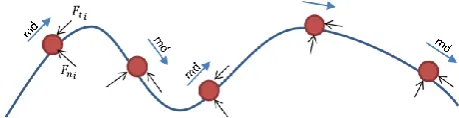
In this study, grinding of a planar work-piece with an unknown shape was investigated, admittance control based active compliance controller was developed and implemented on a robotic – grinding setup. Hybrid controller which controls feedrate in local tangential direction and grinding interaction force in local normal direction was developed. While feedrate compensation was performed with 6 DOF hexapod robot, normal force compensation was performed by high frequency piezo actuator. Local normal and tangential directions are shown in Fig. 1.

With the proposed method in this paper, after providing

Manuscript received July 16, 2017; revised August 2, 2017. This work was supported by Scientific and Technological Research Council of Turkey (TÜBİTAK) under Grant 114E274.

Abdulhamit DONDER is with Middle East Technical University, Mechanical Engineering Department, Ankara, Turkey (e-mail: adonder@ metu.edu.tr).

Erhan ilhan KONUKSEVEN is with Middle East Technical University, Mechanical Engineering Department, Ankara, Turkey. (phone: +90-312-2102540; e-mail: [email protected]).

planarity of the work-piece with the ground, stringent calibration is not needed. In order to obtain constant depth of cut from a homogeneous material, the grinding parameters such as feedrate, spindle speed, should be invariant throughout the surface profile. These requirements can be achieved via hybrid force/velocity control [2].

In [3], the implementation of grinding of a work-piece with an unknown shape was performed using the hybrid force/velocity control structure. The authors dealt with the problems related to configuration dependent dynamics of the manipulator. In [4], the effects of elastic transmission of the robots during contour tracking of a work-piece with an unknown shape was investigated. The large force oscillations due to the elasticities in joints are compensated by an additional normal velocity feedback loop. In [5], decoupling of normal force and tangential velocity control loops was studied. The controller was expressed as multi input – multi output, time varying, PID controller. In [6], joint friction effects to normal force and tangential velocity variations in hybrid force / velocity controller were investigated.

In this study, two different control methods namely proportional - integral – derivative (PID) and active disturbance rejection control (ADRC) were utilized for hybrid force/velocity control. The optimization of controller parameters was done by genetic algorithm. For modelling of the system, system identification techniques were utilized. In this paper, firstly the experimental setup and measurement setup are given in Section II and III. The utilized control structure is given in Section IV; then information about modelling and optimization of controller parameters is given in Section V. After that experiments are explained in Section VI. Finally results, discussion and conclusions are given.

II. EXPERIMENTAL SETUP

In addition to 6-DoF parallel manipulator, the experimental setup has an additional 1-DoF which is actuated by a piezo actuator. The actuator is fixed to the properly constrained table, presents a single degree of freedom in the x direction as shown in Fig. 3. While performing grinding in y direction as shown in the same figure, the machining errors can be reduced by admittance

Fig. 1 Illustration of the grinding operation on a curvy surface

Contour Tracking by Hybrid Force/Velocity

Controlled Grinding: Comparison of Controllers

ADRC - PID

Abdulhamit DONDER and Erhan ilhan KONUKSEVEN

control based negative compensation by the actuation of the piezo actuator. The force/torque sensor is able to measure the data of the forces on 3 Cartesian basis axes and of the torques about the same axes.

The parts shown in Fig. 2 are:

1. Hexapod (6 DoF): It has 6 DoF and is used to move the spindle which carries the tool.

2. ATI Gamma IP60 Force / Torque Sensor 3. Spindle

4. Workpiece (St37) 5. Piezo Actuator

6. Table (which has 1 DoF in x direction as shown in Fig. 3 during machining)

In order to control and drive hexapod, force/torque sensor, piezo actuator and spindle; MATLAB SIMULINK software was utilized. These four devices are connected to the workstation over the protocols summarized in Fig. 4.

Fig. 2 The overall appearance of the test setup. See [7] for detailed explanation about the setup.

Fig. 3 The overall appearance of the test setup and coordinate axes

Fig. 4 Devices and Connection Protocols

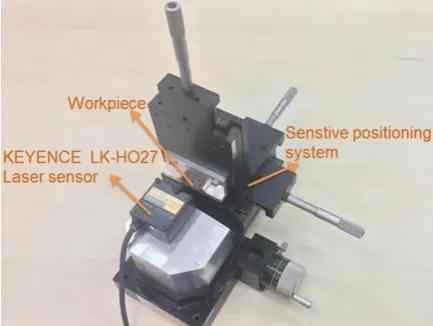
III. SURFACE FORM MEASUREMENT SETUP

In order to understand the form change of the work-piece, it should be measured before and after the experiment. That is why a measurement setup was built as shown in Fig. 5. The measurement system consists of a sensitive positioning system and a laser measurement device. In this system, laser measurement device is located at the fixed part of the positioning system and the work-piece is passed by in front of it. In order to obtain the surface form, a measurement is taken in every 500mintervals.

IV. THE CONTROL STRUCTURE:HYBRID FORCE/VELOCITY

CONTROL

In order to obtain constant depth of cut from variable surface, the key strategy that should be implemented is imposing appropriate normal force and tangential velocity. That is, classical explicit hybrid force/velocity control can be implemented [2]. In order to obtain the actual local normal force from measured X and Y force components the algorithm which is explained in [8] was utilized.

The local tangential force is as follows:

tool zSpindle t

r M

F  (1)

Where: zSpindle

M : Measured moment around Z axis of the spindle tool

r : Radius of the cutting tool

However, with the used setup, measured moment around Z axis of the force/torque sensor MZ is not the moment

around the axis of the spindle since the force/torque sensor has an eccentricity with respect to the spindle. Therefore, local tangential force is calculated as follows:

tool y x z

tool zSpindle t

r

x F y F M

r M

F       (2)

Where: X

F : Measured force in X direction Y

F : Measured force in Y direction

y

 : Eccentricity of the force/torque sensor with respect to spindle axis in Y direction

x

 : Eccentricity of the force/torque sensor with respect to spindle axis in X direction

After calculation of F_t, the local normal force F_n is calculated by the utilization of the following equality:

2 2 2

2

t n Y

X F F F

F    (3)

Therefore:

2 2 2

t y x

n F F F

F    (4)

Velocity control is performed by the controller of the hexapod robot. When the piezo actuator is in action, the resultant feedrate is increases since the feedrate is defined as:

2 2

Pzo Hex

R V V

F   (5)

Where: Hex

V : Velocity of the hexapod Pzo

V : Velocity of the piezo actuator

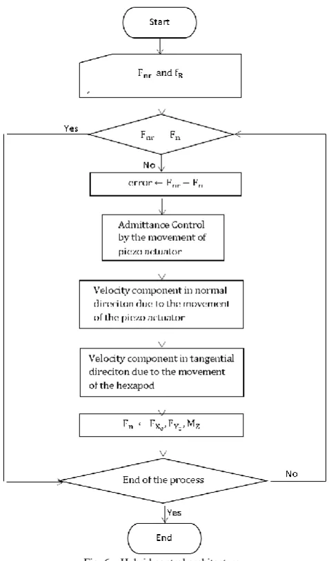
In order to keep the local feedrate constant, the hexapod robot arranges its velocity according to the movements of the piezo actuator. The control structure is illustrated in Fig. 6. Firstly, reference local feedrate and normal force components are entered by the user. If the actual normal force is not equal to the reference normal force, the error is defined as the difference between reference normal force and the actual normal force. In the next step, the actual normal force is controlled by the movements of the piezo actuator. However, due to the movements of it, the feedrate, which is the combination of the movements of the hexapod and the piezo actuator, increases. In order to keep the local feedrate constant, the controller decreases the velocity of the hexapod. After that updated actual normal force is calculated from measured X and Y force components and the moment around Z axis. Control of the feedrate of the hexapod robot is considered as an independent loop[5].

The symbols in Fig. 6 are:Fnr: reference normal force, Fn:

Actual normal force, FX0: X component of the measured

force, FY0: Y component of the measured force, MZ:

Measured moment around Z axis, fR: feedrate in tangential

direction

A. PID Controller

PID Controllers are extensively used in industry due to their simplicity, robustness, easy implementation and their well-known tuning techniques [9]. The most important weaknesses of PID control are as follows [10]:

 Due to noise sensitivity, PID controller is often used without derivative(D) term

 Integral term introduces saturation and reduced stability margin due to phase lag.

B. Active Disturbance Rejection Controller

In order to eliminate the weaknesses of classical PID control, ADRC was firstly proposed in [11], [12]. It has been studied for approximately two decades. ADRC proposes following fundamental properties[10]:

Set-point Jump and Tracking Differentiator: Generally, reference input of the system is given as a step input which is not suitable for most of the dynamic system since it results in a sudden jump of the output. In order to eliminate this drawback, it is necessary to have a transient profile that can be easily followed by the output of the system. The most important utility of this method is the ability to take the derivative of a noisy signal with a good signal to noise ratio and to work as a noise filter.

Fig. 6 – Hybrid control architecture

Nonlinear Feedback Combination: A nonlinear function is proposed for the combination of nonlinear feedbacks.

Total Disturbance Estimation and Rejection via Extended State Observer (ESO): ESO provides real time feedback to eliminate the disturbance by estimating the disturbances and unmodelled dynamics of the system. This structure was designed for robustness against the variations in plant. Therefore, the necessity for integral control which has an inherent lag, that can make a closed loop control system unstable, is eliminated.

V. MODELLING AND OPTIMIZATION OF CONTROLLER

PARAMETERS

For modelling purposes MATLAB SIMULINK was used.

A. System Identification of the Piezo Actuator

- Data Collecting Experiments:

- System Identification:

After the collection of input and output data of the piezo actuator, system identification analysis was performed. For this purpose, MATLAB System Identification Toolbox was utilized[13]. Transfer function model estimation is performed by ARX method[14] by MATLAB System Identification Toolbox. By using each dataset, (input and output couple) 3 discrete transfer functions (2nd, 3rd, 4th order) were estimated. Then the 2nd order transfer function which was estimated by the 3rd dataset was selected:

9503 . 0 949 . 1

001333 . 0 )

( ₂

 



z z

z z

G (6)

B. Overall Model

The unknown shape of the work-piece is designed as sinusoidal. The location of the profile with respect to the tool is updated at each time instant according to the given feedrate. The parameters of the sinusoidal profile are given in Fig. 7.

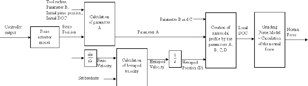
Differentiation of parameter D was used as tool feedrate and A as the position of the piezo actuator. Closed loop controllers were used in the system. The controller output is the position change of the piezo actuator as shown in Fig. 8. After the position of the piezo actuator is determined, “A” parameter of sinusoidal profile is calculated in “Calculation of parameter A” block. Since this “A” parameter determines the distance between the tool and the work-piece in X direction, its inputs are tool radius, amplitude of the profile (B), initial depth of cut and initial piezo position.

“D” value of sinusoidal profile was determined according to piezo velocity. Therefore, in order to determine the piezo velocity, derivative of the piezo position was taken. After that “Calculation of hexapod velocity” block takes set feedrate and piezo velocity as inputs and calculates

Fig. 7 y(t)=A+Bsin(Ct+D) -- C is frequency(rad/sec) w=2f

the hexapod velocity. By taking the integral of this velocity value, parameter “D” was reached.

After determination of all the parameters for sinusoidal profile generation, it was created and Local Depth of Cut-DOC is determined by calculating the intersection point of the tool and the surface profile. The determination of generated normal force component from the local DoC was performed by the grinding force model explained in [15]. After “Plant” block, the loops are closed by adding Gaussian Noise with a variance of 0.8 which is the variance of actual measured force data.

C. Optimization of Controller Parameters by Genetic

Algorithm

Genetic Algorithm is a method by which constructed and unconstructed optimization problems can be solved. At each time step, the algorithm selects some individuals in order to use them as parents in the next iteration. These selected parents are used to generate new generation at the following time step. After a certain iteration, optimal solution is approached. The usage of this method in controller parameter tuning is also extensively used technique[16]– [18]. In this study, genetic algorithm was used for the tuning of controller parameters. For the implementation of genetic algorithm, MATLAB SIMULINK Response Optimization was used[19].

VI. EXPERIMENTS

MATLAB SIMULINK was utilized for controlling the devices of the grinding setup. The “Plant” block without its control part is shown in Fig. 9. In this figure “Controller Input” is the amount of change in the piezo position. After the calculation of the new piezo position, the signal was given to the piezo actuator. In order to calculate the velocity of the hexapod robot, the data which is given to the piezo actuator goes through a derivation block in order to determine the velocity of the piezo actuator. After that the velocity of the hexapod robot is calculated from the set feedrate value with (5). After the grinding operation, the generated force values were obtained and the normal force was calculated.

A. Experiment with PID Controller

The PID parameters were determined by genetic algorithm as: Kp: 84.06, Kd: 14.1, Ki: -0.01766

Fig. 9 Plant Model for Experiment

The experiment parameters are: Set feedrate: 0.1 mm/sec, Spindle speed: 25000 rpm, Material: 4mm ST37

B. Experiment with Active Disturbance Rejection

Controller

The controller parameters were determined by genetic algorithm as: Kp: 61.17, Kd: 78.64, alpha: 0.9448

Additionally, the parameter b0 was taken as 0.5.

The experiment parameters are: Set feedrate: 0.1 mm/sec, Spindle speed: 25000 rpm, Material: 4mm ST37

VII. RESULTS

A. Results of the Experiment with PID Controller

The variation of the local normal force when it is set to 10 N is shown in Fig. 10.

Fig. 10 Local Normal Force (PID)

The movements of the piezo actuator are shown in Fig. 11.

Fig. 11 Piezo Actuator Movements (PID)

The velocity of the piezo actuator after discrete derivation is shown in Fig. 12.

Fig. 12 Piezo Actuator Velocity (PID)

The velocity of hexapod robot is shown in Fig. 13.

Fig. 13 Hexapod Velocity (PID)

The change in the surface form is shown in Fig. 14.

Fig. 14 Surface forms before and after grinding operation (PID)

In order to compare two surface forms, shown in Fig. 14, they were superimposed and mean square error was calculated as 0.000764. In order to eliminate the effects of contact and leaving points, the region between 5mm and 27 mm was considered.

B. Results of the Experiment with ADRC

The variation of the local normal force when it is set to 10 N is shown in Fig. 15.

Fig. 15 Local Normal Force (ADRC)

The movements of the piezo actuator are shown in Fig. 16.

The velocity of the piezo actuator after discrete derivation is shown in Fig. 17.

Fig. 17 Piezo Actuator Velocity (ADRC)

The velocity of hexapod robot is shown in Fig. 18

Fig. 18 Hexapod Velocity (ADRC)

The change in the surface form is shown in Fig. 19.

Fig. 19 Surface forms before and after grinding operation (ADRC)

In order to compare two surface forms, shown in Fig. 19, they were superimposed and the mean square error was calculated as 0.001171. In order to eliminate the effects of contact and leaving points, just the region between 5mm and 27 mm was considered.

VIII. DISCUSSION

The mean square error of the surface profile obtained by ADRC is greater than the surface profile obtained by PID controller. As it is understood from Fig. 11 and, Fig. 16 the work-piece is not well-aligned with respect to the piezo actuator. However, when Fig. 14 and Fig. 19 are considered, misalignment does not seem to cause a problem which is very good advantage of the force control. Additionally, with force control, the disadvantages due to tool wear are eliminated. From piezo and hexapod velocity figures, it can be seen that the local feedrate is kept constant at 0.1 mm/sec.

IX. CONCLUSION

In this study hybrid force/velocity control method was implemented to the robotic grinding experimental setup. While the local normal force was tried to be kept constant by the movements of the piezo actuator, the compensation of the local tangential velocity was performed by the hexapod robot. Two different control algorithms (PID and ADRC) were tried and compared. It was shown that PID method results in better than ADRC.

REFERENCES

[1] R. Bernard and S. Albright, Robot calibration. Springer Science \& Business Media, 1993.

[2] M. H. Raibert and J. J. Craig, “Hybrid Position / Force Control of Manipulators,” J. Dyn. Syst. Meas. Control, vol. 102, no. June 1981, 1981.

[3] F. Jatta, G. Legnani, A. Visioli, and G. Ziliani, “On the use of velocity feedback in hybrid force/velocity control of industrial manipulators,” Control Eng. Pract., vol. 14, no. 9, pp. 1045– 1055, 2006.

[4] F. Jatta, G. Legnani, and A. Visioli, “Hybrid force / velocity control of industrial manipulators with elastic transmissions,” in

Proceedings of the 2003 IEEE/RSJ Int. Conference on Intelligent Robots and Systems, 2003, no. October, pp. 3276–3281. [5] N. Pedrocchi, A. Visioli, G. Ziliani, and G. Legnani, “On the

elasticity in the dynamic decoupling of hybrid force/velocity control in the contour tracking task,” in 2008 IEEE/RSJ Intern. Conf. on Intell. Robots and Sys., IROS, 2008, pp. 955–960. [6] F. Jatta, G. Legnani, and A. Visioli, “Friction Compensation in

Hybrid Force / Velocity Control of Industrial Manipulators,”

IEEE Trans. Ind. Electron., vol. 53, no. 2, pp. 604–613, 2006. [7] K. Açıkgöz, “Predictıon Of The Cutting Forces for Robotic

Grinding Processes with Abrasive Mounted Bits,” Middle East Technical University, 2015.

[8] G. Ziliani, A. Visioli, and G. Legnani, “A mechatronic approach for robotic deburring,” Mechatronics, vol. 17, no. 8, pp. 431–441, 2007.

[9] L. Reznik, O. Ghanayem, and A. Bourmistrov, “PID plus fuzzy controller structures as a design base for industrial applications,”

Eng. Appl. Artif. Intell., vol. 13, no. 4, pp. 419–430, 2000. [10] J. Han, “From PID to active disturbance rejection control,” IEEE

Trans. Ind. Electron., vol. 56, no. 3, pp. 900–906, 2009. [11] J. Han, “Active disturbance rejection control and its application,”

Control Decis., vol. 13, pp. 19–23, 1998.

[12] J. Han, “Nonlinear design methods for control systems,” in 14th IFAC World Congr., 1999.

[13] “MATLAB System Identification Toolbox.” [Online]. Available: https://www.mathworks.com/products/sysid.html. [Accessed: 15-Jun-2017].

[14] M. Verhaegen and V. Verdult, Filtering and System Identification. Cambridge University Press, 2007.

[15] M. L. Navid and E. ilhan Konukseven, “Hybrid model based on energy and experimental methods for parallel hexapod-robotic light abrasive grinding operations,” Int. J. Adv. Manuf. Technol., 2017.

[16] Z. Jinhua, Z. Jian, D. Haifeng, and W. Sun’an, “Self-organizing genetic algorithm based tuning of PID controllers,” Inf. Sci. (Ny)., vol. 179, no. 7, pp. 1007–1018, 2009.

[17] Y. Mitsukura, T. Yamamoto, and M. Kaneda, “A Design of Self-Tuning PID Controllers Using a Genetic Algorithm,” in Proc. of the American Cont. Conf., 1999, no. June, pp. 1361–1365. [18] T. L. Seng, M. Bin Khalid, and R. Yusof, “Tuning of a

Neuro-Fuzzy Controller by Genetic Algorithm,” in IEEE TRANSACTIONS ON SYSTEMS, MAN, AND CYBERNETICS— PART B: CYBERNETICS, 1999, vol. 29, no. 2, pp. 226–236. [19] “Response Optimization SIMULINK.” [Online]. Available: