Branch and Bound Method for Scheduling Precedence Constrained Tasks on Parallel Identical Processors

Branch and Bound Method for Scheduling

Precedence Constrained Tasks on Parallel

Identical Processors

N.S.Grigoreva

Abstract—The multiprocessor scheduling problem is one of the classic NP-hard optimization problems. This paper deals with the problem of scheduling tasks to parallel processors with the goal of minimizing ex-ecution time. The branch and bound algorithm pro-duces a feasible IIT(inserted idle time) schedule for a fixed length T. In order to optimize over T we must iterate the scheduling process over possible values of T. The upper and lower bound on T is defined. New dominance criteria are introduced to curtail the enu-meration tree. By this approach it is generally possi-ble to eliminate most of the useless nodes generated at the lowest levels of decision tree. To illustrate the efficiency of our approach we tested it on randomly generated task graphs.

Keywords: multiprocessor scheduling, parallel proces-sors, Branch and Bound algorithm, IIT (inserted idle time), task graph

1

Introduction

The problem of minimizing the makespan while schedul-ing tasks to parallel identical processors is a classical com-binatorial optimization problem. Following the 3-field classification scheme proposed by Grahamet al. [1], this problem is denoted by P|prec|Cmax. Branch and bound

algorithm is presented for the scheduling problem with tasks have to be executed on several parallel identical processors. This problem relates to the scheduling prob-lem [2,3],it has many applications, and it isN P-hard [4]. Branch and bound method [5,6] allows to obtain an exact solution or, when the number of iterations is restricted, a fairly good approximation of the solution. A new method for evaluating partial solutions, selecting the next task and new ways of reducing the exhaustive search was de-signed. To illustrate the effectiveness of this approach we tested it on randomly generated task graphs.

We consider a system of tasks U = {u1u2, . . . , un}.

The execution time of each task t(ui) is known.

Precedence constructions between tasks are represented by a directed acyclic task graph

∗_{Manuscript accepted March, 21,2014. N.S.Grigoreva is with}

St.Petersburg State University, Department of Mathematics and Mechanics, St.Petersburg,Russia, Email: n.s.grig@gmail.com

G = ⟨U, E⟩. E is a set of directed arcs, an arc

e = (ui, uj) ∈E if and only ifui ≺uj. The expression

ui ≺ uj means that the task uj may be initiated only

after completion of the taskui. Set of tasks is performed

on parallel identical processors, any task can run on any processor and each processor can perform no more than one task at a time. Task preemption is not allowed. The usual objective function is completion time of the scheduled task graph also referred to as makespan or schedule length.

For this model, we can consider two problems. In the first problem the number of processors m is known and the goal is to minimize the execution time - makespan. In the second one the makespan is known, the goal is to minimize the number of processors. To solve these two problems, we can apply the same algorithm.

Subtask of these two problems is the task of constructing a feasible schedule for the given number of processors and the given execution time. A schedule for a task setU is the mapping of each task ui ∈ U to a start time τ(ui)

and a processor num(ui). Length of schedule S is the

quantity

TS = max{τ(ui) +t(ui)|ui∈U}.

To solve this problem we apply the branch and bound method in conjunction with binary search. Branch and bound method constructs a feasible scheduleS of length

T for m processors. The algorithm may be used in a binary search mode to find the smallest number of pro-cessors or the smallest makespan. First we propose an approximate IIT algorithm named CP/IIT (critical path/ inserted idle time). Then by combining the CP/IIT al-gorithm and B&B method this paper presents BB/IIT algorithm which can find optimal solutions to parallel scheduling problem.

2

Approximate algorithm

V.Sridharam [7] as a feasible schedule in which a proces-sor is kept idle at a time when it could begin processing a task. We propose an approximate IIT algorithm named CP/IIT (critical path/ inserted idle time).

For each task ui, we define the earliest starting time

vmin(ui) and the latest start time vmax(ui). The

earli-est starting time is numerically equal to the length of the maximal path in the graph Gfrom the initial vertex to the vertex ui. The latest start time vmax(ui) of task ui,

is numerically equal to the difference between the length of the required scheduleTS and the length of the

maxi-mal path from the taskui,to the final vertex. The latest

start timevmax(ui) of taskui is a priority of task. Letk

tasks are put in the schedule and partial schedule Sk is

constructed.

Let be timek[i] the time of the termination of the

pro-cessor i after completion all its tasks. The approximate schedule is constructed by CP/IIT algorithm as follows:

1. Determine the processorl0such as

tmin(l0) = min{timek[i]|i∈1..m}

2. Select the task u0, such as all its predecessors are included in the schedule and

vmax(u0) = min{vmax(ui)|ui∈/Sk}

3. If r0 =vmin(u0)−tmin(l0)>0 then choose a task

u∗∈/ Sk, which can be executed during the idle time

of processor without increasing the start time of the tasku0, namelyvmin(u∗) +t(u∗)≤vmin(u0). 4. If the tasku∗is found, then we assign the tasku∗to

the processor l0 otherwise we assign the task u0 to the processorl0.

In order to examine the effectiveness of CP/IIT algorithm we tested it on randomly generated task graph. The re-sults are shown in Table 1.

3

Branch

and

bound

method

for

constructing

a

feasible

schedule

BB

(

U, T, m

;

S

)

For the formal description of the branch and bound method we must give a definition of partial solutions. It is convenient to represent the schedule as a permu-tation of jobs. For each permutation of tasks π = (ui1, ui2, . . . , uin),one can construct a scheduleSπas

fol-lows: to find the earliest time of the release of processors

tmin, to find the processor that was released at this time,

then the task is assigned to the processor at the earliest possible time, but not before tmin, then every

permuta-tion will uniquely identify the schedule Sπ. Partial

so-lution σk, where k the number of jobs will be regarded

as a partial permutationσk= (ui1, ui2, . . . , uik), which is

determined partial schedule.

Definition 1 The solution γn = (l1, l2, . . . , ln) is called

the extension of partial solutions σk = (q1, q2, . . . , qk), if

l1=q1, l2=q2, . . . , lk =qk.

Definition 2 A partial solution σk is called a feasible if

there exists an extension ofσk, which is a feasible

sched-ule.

For each task ui, we define the earliest starting time

vmin(ui) and the latest start timevmax(ui). In order to

make the feasible schedule, it is necessary that each task

ui∈U,the start time of its executionτ(ui) satisfies the

inequality

vmin(ui)≤τ(ui)≤vmax(ui).

In order to describe the branch and bound method it is necessary to determine the set of tasks that we need to add to a partial solution, the order in which task will be chosen from this set and the rules that will be used for eliminating partial solutions.

3.1

Selection of task

Let I be the total idle time of processors in a fea-sible schedule S of length TS for m processors, then

I = m·TS −

∑n

i=1t(ui). For a partial solution σk we

knowr(ui)— idle time of processor before start the task

ui. Let Ik be the remaining pool of idle for a partial

solution σk. Then Ik = I −

∑k

i=1r(ui). We know the

completion time of processors timek[1 : m]. Denote

tmin(k) = min{timek[i]|i ∈ 1 : m} then tmin(k) is the

earliest time of ending all tasks were included in a partial solutionσk.

At each levelkwill be allocated a set of tasks Uk, which

we call the possible assignments. These are tasks that need to add to a partial solution σk−1, so check all the

possible continuation of the partial solutions.

Definition 3 Task u /∈σk is called the ready task at the

level k, if all its predecessors were included in the partial solutionσkand the earliest starting timevmin(u)satisfies

the inequality vmin(u)−tmin(k)≤Ik.

Task selection procedure Select(Uk, tmin(k);u0)

From the set Uk we choose task u0 with the minimum latest start time. If before beginning this task proces-sor will be idle we are trying to find a task that can be performed during idle time of processor.

1. Select the tasku0, such as

vmax(u0) = min{vmax(ui)|ui∈Uk}.

2. If r0 = vmin(u0)−tmin(k) > 0 then choose a task

u∗∈Uk, which can be executed during the idle time

3. If the tasku∗is found, then we assign the tasku∗to the processor otherwise we assign the tasku0to the same processor.

3.2

Deleting of invalid partial solutions

The main way of reducing of the exhaustive search will be the earliest possible identification unfeasible solutions.

Definition 4 Let the task ucr ∈/ σk is such as

vmax(ucr) = min{vmax(u)|u /∈ σk}. The task ucr ∈/ σk

is called the delayed task forσk, if vmax(ucr)< tmin(k).

Lemma 1 Let delayed task ucr for a partial solution

σk=σk−1∪uk exists, then:

1. The partial solutionσk is unfeasible.

2. For any task u∈Uk, such that

max{tmin(k−1), vmin(u)}+t(u)> vmax(ucr)a

par-tial solutionσk−1∪uis unfeasible.

3. If vmax(uk)< tmin(k)and

tmin(k−1) +t(ucr) > vmax(uk), then the partial

solution σk₋1 is unfeasible.

Another method for determining unfeasible partial solu-tions based on a comparison of resource requirements of tasks and total processing power. In this case we propose to modify the algorithm for determining the interval of concentration [8] for the complete schedule. We apply this algorithm to a partial scheduleσk and determine its

admissibility.

We consider time intervals [t1, t2] ⊆ [tmin(k), TS]. Let

M P(t1, t2) be the total time of free processors in time interval [t1, t2] then

M P(t1, t2) =

m

∑

i=1

max{0,(t2−max{t1, timek[i]})}.

For all task ui ∈/ σk we find minimal time of its

be-gin: v(ui) = max{vmin(ui), tmin(k)}. Let L([t1, t2]) be a length of time interval [t1, t2].

LetMk(t1, t2) be the total minimal time of tasks in time interval [t1, t2],then

Mk(t1, t2) =

∑

ui∈/σk

min{L(xk(ui)), L(y(ui))},

where

xk(ui) = [v(ui), v(ui) +t(ui)]∩[t1, t2],

y(ui) = [vmax(ui), vmax(ui) +t(ui)]∩[t1, t2].

Let

est(σk) = max

[t1,t2]∈[tmin(k),TS]

{Mk(t1, t2)−M P(t1, t2).}

Lemma 2 If est(σk) > 0 then a partial solution σk is

unfeasible.

The pseudo-code of Branch and bound method for con-structing a feasible schedule BB(U, T, m;S) is shown in Algorithm 1.

Algorithm 1BB/IIT algorithm

1: Setk:= 1;time[i] = 0;i∈1 :m;σ0=∅;

2: while(k >0)and (k < n+ 1)do

3: Determine the processor l0 such as tmin(l0) = min{(timek[i]|i∈1..m)}

4: Determine the task ucr such as vmax(ucr) =

min{vmax(u)|u /∈σk−1};

5: if vmax(ucr)≤tmin(l0) then

6: ComputeEST =est(σk−1);

7: if EST ≤0 then

8: Select the task u0, use procedure

Select(Uk, tmin(k);u0)

9: Set the tasku0on processorl0and create par-tial solution σk =σk−1∪u0

10: else

11: Perform step back and create partial schedule

σk−1

12: else

13: There is delayed taskucr. Delete all unfeasible

partial solution by using Lemma 1

14: end if

15: end if

16: end while

17: if k= 0,then

18: Makespan of optimal schedule is greater thenTS.

19: end if

20: if k=n,then

21: We find feasible scheduleS=σn and its makespan

is equalTS

22: end if

4

Computation result

To test method and efficacy evaluations we conducted computational experiment. In the computational experi-ment, we intended to test theBB/IIT algorithm and to test the effectiveness of methods to remove invalid par-tial solutions. For branch and bound method to build a feasible solution, it had to accomplish the task in less than 60 seconds. If a feasible schedule S of length T

problems, but whether or not the solutions obtained are exact or approximate remains an open question. There-fore, the quality of the solutions was estimated against to the lower estimate of the makespan LB. Lowbound LB

of length optimal schedule is

LB= max{tcp,⌈ n

∑

i=1

t(ui)/m⌉},

where tcp is the length critical path in task graph. To

illustrate the effectiveness of our algorithm we tested it on two types graphs.

In the first group a set of task graph were generated using a random task graph generator with 50, 100,150 tasks. The processing time of the tasks has been cho-sen randomly from the interval [1:50]. In the second one we used Standard Task Graph Set which is available at http://www.kasahara.elec.waseda.ac.jp/schedule/.

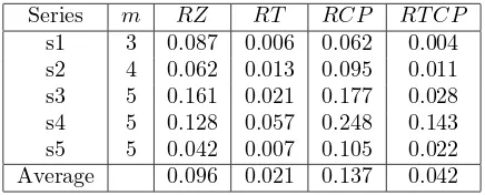
In the first group we divided all tests on 5 series. There are 100 tests in series. We compare the length Z0 of initial solution (obtained by CP/IIT algorithm) and the lengthZCP of initial solution obtained by CP algorithm.

Comparative results are presented in Table 1. The first column of this table contains the name of series tests, in the second one m is a number of processors. The third one contains the relative error of initial solution

RZ = (Z0−LB)/LB and the fourth one contains the relative errorRT = (T−LB)/LB,whereT is the length of schedule obtained by BB/IIT algorithm. Then the fifth column contains the relative error of initial solution

RCP = (ZCP −LB)/LB and the the last one contains

the relative errorRT CP = (TCP −LB)/LB whereTCP

is the the length of schedule obtained by B&B algorithm with select procedure CP.

Table I. Average data for any series of tests.

Series m RZ RT RCP RT CP

s1 3 0.087 0.006 0.062 0.004 s2 4 0.062 0.013 0.095 0.011 s3 5 0.161 0.021 0.177 0.028 s4 5 0.128 0.057 0.248 0.143 s5 5 0.042 0.007 0.105 0.022 Average 0.096 0.021 0.137 0.042

Approximate solution with the error RZ of less then 10 percent in average were obtained by CP/IIT algo-rithm. The average relative error of schedules obtained by BB/IIT algorithm is equal 2 percent.

Table 2 shows the results (percent of optimal solutions found) for the first group of instances. The columnNopt

shows the cases (in percents) where optimal schedules were obtained by BB/IIT method. The next column

shows the number of cases (in percents) in which approx-imate solutions within the error of 0.05 were obtained, but optimal solutions could not be obtained because of CPU time limit. But an intermediate solution can be an optimal solution. The next two columns shows the num-ber of cases in which RT ∈ (0.05,0.1] and RT greater then 0.1.

Table II. Results for the relative error of makespan of schedule.

Series m Nopt RT <0.05 RT <0.1 RT >0.1

s1 3 56 26 14 4

s2 4 70 19 11 0

s3 5 61 23 15 1

s4 5 57 29 11 0

s5 5 69 30 17 3

Average 62.6 23.4 13.6 1.6

It is seen from Table 2 that optimal solution were ob-tained for 63 percent (in average) of the cases tested. For 86 percent of the cases approximate solutions having er-ror of less than 5 percent were obtained.

In the second group of tests we use tests from Standard Task Graph Set. Standard Task Graph Set is a kind of benchmark for evaluation of multiprocessor schedul-ing algorithms, where optimal decisions are known. We considered tests from Standard Task Graph Set with n= 50 and n=100, where n is the number of tasks. Optimal schedules were found byBB/IITalgorithm in 95 percent tests with n=50 and in 89 percent tests with n=100.

5

Conclusion

In this work we proposed a new branch and bound method for solving the multiprocessor scheduling prob-lem of makespan minimization. We also presented a new approximate IIT (inserted idle time) algorithm. We found that the minimum execution time multiprocessor scheduling problem can be solved within reasonable time for moderate-size systems. With an increasing number of tasks, branch and bound method requires more time to obtain the optimal solution. Limiting the number of iterations seems justified and promising way to obtain a good approximate solution. Computer experiment con-firmed efficiency of branch and bound method with this restriction.

References

[1] Graham,R.L.,Lawner E.L., Lenstra J.K.,and Rin-nooy Kan. “Optimization and approximation in de-terministic sequencing and scheduling: A survey”

[2] Computer and job-shop scheduling theory, Ed. by E.G.Coffman, John Wiley,1976.

[3] Brucker P.Scheduling Algorithms, Springer.1997.

[4] Ullman J.D. “NP-complete scheduling problems”

Journal Comput.System Sci.1975. 10. pp. 384–393.

[5] Kasahara H., Narita S. “Practical multiprocessor scheduling algorithms for efficient parallel process-ing”, IEEE Tranzactions on computers.1984,V4. pp.22–33, No.11

[6] Grigoreva N.S., “Branch and bound algorithm for multiprocessor scheduling problem”, Vestnic SP-bGU.seria 10. 2009. Iss.1 pp.44–55.[ in Russian]

[7] Kanet J.J.,Sridharan V., “Scheduling with inserted idle time: problem taxonomy and literature re-view”,Operation Research.2000.V48.Iss.1. pp. 99– 110.

[8] Fernandez E. and Bussell B., “Bounds the number of processors and time for multiprocessor optimal schedules”,IEEE Trans. on Computers.1973.pp.745– 751.

[9] Graham R.L., “Bounds for certain multipro-cessing Anomalies”,Bell System Tecnical journal