SwatCS: Combining simple classifiers with estimated accuracy

SwatCS: Combining simple classifiers with estimated accuracy

Sam Clark and Richard Wicentowski

Department of Computer Science Swarthmore College Swarthmore, PA 19081 USA

[email protected]@cs.swarthmore.edu

Abstract

This paper is an overview of the SwatCS system submitted to SemEval-2013 Task 2A: Contextual Polarity Disambiguation. The sen-timent of individual phrases within a tweet are labeled using a combination of classifiers trained on a range of lexical features. The classifiers are combined by estimating the ac-curacy of the classifiers on each tweet. Perfor-mance is measured when using only the pro-vided training data, and separately when in-cluding external data.

1 Introduction

Spurred on by the wide-spread use of the social net-works to communicate with friends, fans and cus-tomers around the globe, Twitter has been adopted by celebrities, athletes, politicians, and major com-panies as a platform that mitigates the interaction be-tween individuals.

Analysis of this Twitter data can provide insights into how users express themselves. For example, many new forms of expression and language fea-tures have emerged on Twitter, including expres-sions containing mentions, hashtags, emoticons, and abbreviations. This research leverages the lexical features in tweets to predict whether a phrase within a tweet conveys a positive or negative sentiment.

2 Related Work

A common goal of past research has been to discover and extract features from tweets that accurately in-dicate sentiment (Liu, 2010). The importance of

feature selection and machine learning in sentiment analysis has been explored prior to the rise of so-cial networks. For example, Pang and Lee (2004) apply machine learning techniques to extracted fea-tures from movie reviews.

More recent feature-based systems include a lexicon-based approach (Taboada et al., 2011), and a more focused study on the importance of both ad-verbs and adjectives in determining sentiment (Be-namara et al., 2007). Other examples include us-ing looser descriptions of sentiment rather than rigid positive/negative labelings (Whitelaw et al., 2005) and investigating how connections between users can be used to predict sentiment (Tan et al., 2011).

This task differs from past work in sentiment anal-ysis of tweets because we aim to build a model capa-ble of predicting the sentiment of sub-phrases within the tweet rather than considering the entire tweet. Specifically, “given a message containing a marked instance of a word or a phrase, determine whether that instance is positive, negative or neutral in that context” (Wilson et al., 2013). Research on context-oriented polarity predates the emergence of social networks: (Nasukawa and Yi, 2003) predict senti-ment of subsections in a larger docusenti-ment.

N-gram features, part of speech features and “micro-blogging features” have been used as accu-rate indicators of polarity (Kouloumpis et al., 2011). The “micro-blogging features” are of particular in-terest as they provide insight into how users have adapted Twitter tokens to natural language to por-tray sentiment. These features include hashtags and emoticons (Kouloumpis et al., 2011).

3 Data

The task organizers provided a manually-labeled set of tweets. For parts of this study, their data was sup-plemented with external data (Go et al., 2009).

As part of pre-processing, all tweets were part-of-speech tagged using the ARK TweetNLP tools (Owoputi et al., 2013). All punctuation was stripped, except for #hashtags, @mentions, emoticons :), and exclamation marks. All hyper-links were replaced with a common string, “URL”.

3.1 Common Data

The provided training data was a collection of ap-proximately 15K tweets, manually labeled for senti-ment (positive, negative, neutral, or objective) (Wil-son et al., 2013). These sentiment labels applied to a specific phrase within the tweet and did not necessarily match the sentiment of the entire tweet. Each tweet had at least one labeled phrase, though some tweets had multiple phrases labeled individu-ally. Overall, 37% of tweets had one labeled phrase, with an average of 2.58 labeled phrases per tweet.

Each of our classifiers were binary classifiers, la-beling phrases as either positive or negative. As such, approximately 10.5K phrases labeled as objec-tive or neutral were pruned from the training data, resulting in a final training set containing 5362 la-beled phrases, 3445 positive and 1917 negative.

The test data consisted of tweets and SMS mes-sages, although the training data contained only tweets. The test set for the phrase-level task (Task A) contained 4435 tweets and 2334 SMS messages.

3.2 Outside Data

Task organizers allowed two submissions, a con-strained submission using only the provided training data, and an unconstrained submission allowing the use of external data. For the unconstrained submis-sion, we used a data set built by Go et al. (2009). The data set was automatically labeled using emoticons to predict sentiment. We used a 50K tweet subset containing 25K positive and 25K negative tweets.

3.3 Phrase Isolation

For tweets containing a single labeled phrase, we use the entire tweet as the context for the phrase. For tweets containing two labeled phrases, we use the

unigram label bigram label happy pos not going neg

good pos looking forward pos great pos happy birthday pos love pos last episode neg best pos i’m mad neg

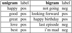
Table 1: The 5 most influential unigram and bigrams ranked by information gain.

context from the start of the tweet to the end of the first phrase as the context for the first phrase, and the context from the start of the second phrase to the end of the tweet for the second phrase. If more than two phrases are present, the context for any phrase in the middle of the tweet is limited to only the words in the labeled phrase.

4 Classifiers

The system uses a combination of naive Bayes clas-sifiers to label the input. Each classifier is trained on a single feature extracted from the tweet. The classi-fiers are combined using a confidence-weighted vot-ing scheme. The system applies a simple negation scheme to all of the language features used by the classifiers. Any word following a negation term in the phrase has the substring “NOT” prefixed to it. This negation scheme was applied to n-gram fea-tures and lexicon feafea-tures.

4.1 N-gram Features

Rather than use all of the n-grams as features, we ranked each n-gram (w/POS tags) by calculating its chi-square-based information gain. The top 2000 n-grams (1000 positive, 1000 negative) are used as features in the n-gram classifier. Both a unigram and bigram classifier use these ranked (word/POS) fea-tures. Table 1 shows the highest ranked unigrams and bigrams using this method.

4.2 Sentiment Lexicon Features

0.78 0.8 0.82 0.84 0.86 0.88 0.9 0.92 0.94 0.96 0.98

0 0.1 0.2 0.3 0.4 0.5 0.6 0.7 0.8 0.9

Confidence/classifier accuracy

alpha = abs(P(pos) - P(neg)) Alpha vs. Classifier accuracy

Figure 1: Classifier accuracy increases as the difference between the probabilities of the labelings increases.

4.3 Part of Speech and Special Token Features

Three additional classifiers were built using features extracted from the tweets. Our third classifier uses only the raw counts of specific part of speech tags: adjectives, adverbs, interjections, and emoticons. The fourth classifier uses the emoticons as a fea-ture. To reduce the noise in the emoticon feature set, many (over 25) different emoticons are mapped to the basic “:)” and “:(” expressions. Some emoticons such as “xD” did not map to these basic expressions. A fifth classifier gives added weight to words with extraneous repeated letters. Words containing two or more repeated letters (that are not in a dictionary, e.g. “heyyyyy”, “sweeeet”) are mapped to their pre-sumed correct spelling (e.g. “hey”, “sweet”).

5 Confidence-Based Classification

To combine all of the classifiers, the system esti-mates the confidence of each classifier and only ac-cepts the classification output if the confidence is higher than a specified baseline. To establish a clas-sifier’s confidence, we take the absolute value of the difference between a classifier’s positive output probability and negative output probability, which we call alpha. Alpha values close to 1 indicate high confidence in the predicted label; values close to 0 indicate low confidence in the predicted label.

5.1 Classifier Voting

The predicted accuracy of each classifier is deter-mined after the trained classifiers are evaluated us-ing a development set with known labels. Usus-ing the dev set, we calculate the accuracy of each

classi-rank classifier data polarity acc

1 unigrams (C) positive 0.89 2 unigrams (U) positive 0.88 3 lexicon (C) negative 0.83 4 lexicon (U) negative 0.81 5 tagcount (C) positive 0.78 6 bigrams (C) positive 0.75 7 tagcount (U) novote <0.65 8 bigrams (U) novote <0.65

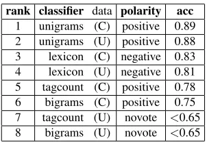
Table 2: An example of the polarity and corresponding accuracy output for each classifier for a single tweet. The labels (C) and (U) indicate whether the classifier was trained on constrained training data or on unconstrained data (Go et al., 2009).

fier at alpha values between 0 and 1. The result is a trained classifier with an approximation of overall classification accuracy at a given alpha value. Fig-ure 1 shows the relationship between alpha value and overall classifier accuracy. As expected, classi-fication accuracy increases as confidence increases.

Table 2 shows the breakdown of classifier accu-racy for a single tweet using both provided and ex-ternal data. The accuracy listed is the classifier-specific accuracy determined by the alpha value for that phrase in the tweet. Using a dev set, we ex-perimentally established the most effective baseline to be 0.65. In the voting system described below, only classifiers with confidence above the baseline (per marked phrase) are used. Therefore, the spe-cific combination of classifiers used for each phrase may be different.

An unlabeled phrase is assigned a polarity and confidence value from each classifier. These proba-bilities are combined using a voting system to deter-mine a single output. This voting system calculates the final labeling by computing the average proba-bility for each label only for those classifiers with estimated accuracies above the baseline. The label with the highest overall probability is selected.

6 Results

unigram label bigram label lexicon label aint neg school tomorrow neg bad neg excited pos not going neg excited pos sucks neg didn’t get neg tired neg sick neg might not neg dead neg poor neg gonna miss neg poor neg smh pos still haven’t neg happy pos tough pos breakout kings neg black neg greatest pos work tomorrow neg good pos f*ck neg ray lewis pos hate neg nets neg can’t wait pos sorry neg

Table 3: The most influential features from the unigram, bigram, and lexicon classifiers.

evaluated using the Twitter and SMS data described in Section 3.1. As mentioned, our system used a bi-nary classifier, predicting only positive and negative labels, making no neutral classifications.

The constrained system evaluated on the Twitter test set had an F-measure of .672, with a high dis-parity between the F-measure for tweets labeled as positive versus those labeled as negative (.79 vs .53). The unconstrained system on the Twitter test set un-derperformed our constrained system, with an F-measure of only .639.

The constrained system on the SMS test set yielded an F-measure of .660; the unconstrained sys-tem on the same data yielded an F-measure of .679.

6.1 Features Extracted

The most important features extracted by the un-igram, bigram and lexicon classifiers are shown in Table 3. Features such as “ray lewis”, “smh”, “school tomorrow”, “work tomorrow”, “breakout kings” and “nets” demonstrate that the classifiers formed a relationship between sentiment and collo-quial language. An example of this understanding is assigning a strong negative sentiment to “sucks” (as the verb “to suck” does not carry sentiment). The bi-grams “breakout kings”, “ray lewis” and “nets” are interesting features because their sentiment is highly cultural: “breakout kings” is a popular TV show that was canceled, “ray lewis” a high profile player for an NFL team, and “nets” a reference to the strug-gling NBA basketball team. Expressions such as “smh” (a widely-used abbreviation for “shaking my head”) show how detecting tweet- and SMS-specific language is important to understanding sentiment in

this domain.

7 Discussion

This supervised system combines many features to classify positive and negative sentiment at the phrase-level. Phrase-based isolation (Section 3.3) limits irrelevant context in the model. By estimat-ing classifier confidence on a per-phrase basis, the system can prioritize confident classifiers and ignore less-confident ones before combination.

Similar results on the Twitter and SMS data sets indicates the similarity between the domains. The external data improved the system on the SMS data and reduced system accuracy on the Twitter data. This difference in performance may be an indication that the supplemental data set was noisier than we expected, or that it was more applicable to the SMS domain (SMS) than we anticipated.

There was a noticeable difference between pos-itive and negative classification accuracy for all of the submissions. This difference is likely due to ei-ther a positive bias in training set used (the provided training data is 64% positive, 36% negative) or a se-lection of features that favored positive sentiment.

7.1 Improvements and Future Work

Unfortunately, the time constraints of the evalua-tion exercise led to a programming bug that wasn’t caught until after the submission deadline. In pre-processing, we accidentally stripped most of the emoticon features out of the text. While it is un-clear how much this would have effected our final performance, such features have been demonstrated as valuable in similar tasks. After fixing this bug the system performs better in both constrained and unconstrained situations (as evaluated on the devel-opment set).

References

Farah Benamara, Carmine Cesarano, Antonio Picariello, Diego Reforgiato, and V Subrahmanian. 2007. Senti-ment analysis: Adjectives and adverbs are better than adjectives alone. InProceedings of the International Conference on Weblogs and Social Media (ICWSM). A. Go, R. Bhayani, and Huang. L. 2009. Twitter

senti-ment classification using distant supervision. Techni-cal report, Stanford University.

Efthymios Kouloumpis, Theresa Wilson, and Johanna Moore. 2011. Twitter sentiment analysis: The good the bad and the omg. InProceedings of the Fifth In-ternational AAAI Conference on Weblogs and Social Media, pages 538–541.

Bing Liu. 2010. Sentiment analysis and subjectivity.

Handbook of natural language processing, 2:568. Tetsuya Nasukawa and Jeonghee Yi. 2003. Sentiment

analysis: capturing favorability using natural language processing. InProceedings of the 2nd international conference on Knowledge capture, K-CAP ’03, pages 70–77.

Olutobi Owoputi, Brendan O’Connor, Chris Dyer, Kevin Gimpel, Nathan Schneider, and Noah A. Smith. 2013. Improved part-of-speech tagging for online conver-sational text with word clusters. In Proceedings of NAACL 2013.

Bo Pang and Lillian Lee. 2004. A sentimental edu-cation: sentiment analysis using subjectivity summa-rization based on minimum cuts. In Proceedings of the 42nd Annual Meeting on Association for Compu-tational Linguistics, ACL ’04, Stroudsburg, PA, USA. Association for Computational Linguistics.

Maite Taboada, Julian Brooke, Milan Tofiloski, Kimberly Voll, and Manfred Stede. 2011. Lexicon-based meth-ods for sentiment analysis. Computational linguistics, 37(2):267–307.

Chenhao Tan, Lillian Lee, Jie Tang, Long Jiang, Ming Zhou, and Ping Li. 2011. User-level sentiment anal-ysis incorporating social networks. InProceedings of the 17th ACM SIGKDD international conference on Knowledge discovery and data mining, pages 1397– 1405.

Casey Whitelaw, Navendu Garg, and Shlomo Argamon. 2005. Using appraisal groups for sentiment analysis. In Proceedings of the 14th ACM international con-ference on Information and knowledge management, CIKM ’05, pages 625–631.

Janyce Wiebe, Theresa Wilson, and Claire Cardie. 2005. Annotating expressions of opinions and emotions in language.Language Resources and Evaluation, 39(2-3):165–210.

Theresa Wilson, Zornitsa Kozareva, Preslav Nakov, Sara Rosenthal, Veselin Stoyanov, and Alan Ritter. 2013.