On a Dynamic Optimization Technique for Resource Allocation Problems in a Production Company

(1)

On a Dynamic Optimization Technique for Resource

Allocation Problems in a Production Company

Chuma R. Nwozo1, Charles I. Nkeki2

1_{Department of Mathematics, University of Ibadan, Ibadan, Nigeria} 2_{Department of Mathematics, University of Benin, Benin City, Nigeria}

Email: [email protected], [email protected]

Received May 7, 2012; revised June 10, 2012; accepted June 24, 2012

ABSTRACT

This paper examines the allocation of resource to different tasks in a production company. The company produces the same kinds of goods and want to allocate m number of tasks to 50 number of machines. These machines are subject to breakdown. It is expected that the breakdown machines will be repaired and put into operation. From past records, the company estimated the profit the machines will generate from the various tasks at the first stage of the operation. Also, the company estimated the probability of breakdown of the machines for performing each of the tasks. The aim of this paper is to determine the expected maximize profit that will accrue to the company over T horizon. The profit that will

accrued to the company was obtained as N4,571,100,000 after 48 weeks of operation. At the infinty horizon, the

profit was obtained to be N20,491,000,000. It was found that adequate planning, prompt and effective maintainance can enhance the profitability of the company.

Keywords: Dynamic Optimization; Resource Allocation; Company; Machines; Tasks

1. Introduction

We consider the allocation of tasks to different machines in a production company. A certain number of machines is proposed to be purchased at the beginning of a planning horizon. From statistics, the company has an esti- mate of the profit each tasks is to yield at the first stage of operation. Also, the company estimates the probability of breakdown of the machines allocated to each tasks. When a machine breaks down, it goes in for repairs after which it returns to the factory for re-allocation at the beginning of the next period.

In this paper, we formulate the problem as a dynamic optimization (DO). Our approach builds on previous re- search. [1] used the stochastic programming technique of dynamic Programming in financial asset allocation problems for designing low-risk portfolios. [2] proposed the idea of using a parsimonious sufficient static in an appli- cation of approximate dynamic programming to invent- tory management. [3] described an algorithm for com- puting parameter values to fit linear and separable con- cave approximations to the value function for large-scale problems in transportation and logistics. [4] described a more complicated variation of the algorithm that im- plores execution time and memory requirements. The improvement is critical for practical applications to real- istic large-scale problems. [5] used DO for large-scale

asset management problems for both single and multiple assets. [6] extended an approximate DO method to opti- mize the distribution operations of a company manufac- turing certain products at multiple production plants and shipping to different customer locations for sales. [7] considered the allocation of buses from a single station to different routes in a transportation company in Nigeria.

In this section, we consider the methodology adopted in this paper. We start with the problem formulation.

2. Problem Formulation

(2)

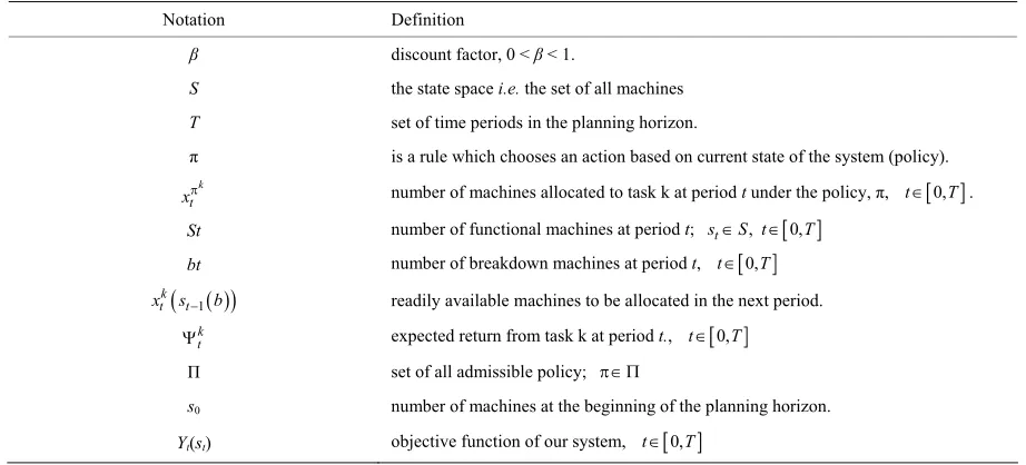
in Table 1.

In the next subsection, we define the one-period expected profit function and formulate the problem as a dynamic program.

3. The Objective and One-Period Expected

Profit Function

If the profit for allocating the k task to the machines at period t is t , the state of the machines is st, number of

machines allocated to operate on task k at period t under policy π, is _tk

k



x

 







1



k

t t t

and the number of break down machines is bt, then the profit that will accrue to the company over

T-horizon is given by

0 1

T m k

t k

x s b



 







1



k

t t

x s_ b

 

 

 

0,1, ,

 





.

The expected maximum profit that will accrue to the company under policy π is given by

 

_{ }

0 1

max

t t

T m t k

t t t

x X s t k

s E 

 

 _ _

 



 (1)

subject to

 



1



1

, k

m

t t t

K

x s b s

 



 t  T

; 1, ,

(2)

0, 1, ,

k

t

x  t T k  m

Note: X(st) is the set of possible solution of problem

(1). Conditioning (1) on s_tS. We now have the

following optimization problem (3)

 



 

Problem (1.3) maximizes the expected profit over X(st)

subject to





' 1 1

max k

t t

T m t k

t t t x X s _{t t k}

s

E _  x



    _ _



 





s b st St

   _ 

 

 



 

 



1



1

, 0,1, ,

k

m

t t t

k

. (3)

x s b s t T

 

 





:S R

For the profit function   

 

1

m k

T T T T

k

, if we accumulate the profit of the first T-stage and add to it the terminal profit

s s



 





 



 



 

,

then (3) becomes

1

' 1 1

max T m t k k

t t t t t

x X s _{t t k} T

T T t

s E x s b

s s S





 

 

   _ _

  

     

 





  _{ }



 





' 1

1

, 0,1, ,

k

m

t t t

k

(4)

x s b s t T



 





0, 1, , ; 1, ,

k

t

. subject to

t T k m

 _ _ _ _ _

k

P x

1

, 1, 2, ,

m k k t k

P x t T







x .

4. Dynamic Programming Formulation and

Optimality

Using st as the state variable at period t and S as the state

space, we can formulate the problem as a dynamic

pro-gram. The number of breakdown machines for task k at

period t is given by k t , where Pk is the probability of

break down machines for task k. Hence, total number of break down machines for all the tasks is given by

.

[image:2.595.309.538.189.340.2]

We therefore have that

Table 1. Notations and their Definitions. Notation Definition

β discount factor, 0 < β< 1.

S the state space i.e. the set of all machines

T set of time periods in the planning horizon.

π is a rule which chooses an action based on current state of the system (policy).

  k

t

x number of machines allocated to task k at period t under the policy, π, t0,T . St number of functional machines at period t; stS t,  0,T

bt number of breakdown machines at period t, t 0,T

k



_{ }



1

t t

x s_ b

k t



readily available machines to be allocated in the next period.

expected return from task k at period t., t 0,T

Π set of all admissible policy; 

s0 number of machines at the beginning of the planning horizon.

[image:2.595.67.528.528.737.2]

(3)

1

m k

t k t

k

b P x





, 1, ,

k k t

.

Let st be the number of machines to be allocated in pe-

riod t and let α be the percentage of break down (but repaired) machines that are expected to join the functional ones in period t, then the transformation equation for the system is given by





1

1 m

t t

k

s s_  P



  



x t  T

, 1, , k

k t

. (5)

Observe that the transformation equation is a random variable.

We now set 1 – α = β in (5) to have,

1 1

m

t t k

s s  P



 



x t   T

 









. (6)

In this case, the optimal policy can be found by comput-ing the value functions through the optimization problem

 





1 k

t t

1

max t

m k

t t t

x _{X s k}

t t

F s x

E F s

_





 s b

S s

 



 

, 1, 2, , . t

(7)

subject to

 



1



1 k

m

t t k

x s b s

 



 t T

, , ;T _t 0

    

; 1, ,

Equivalently,

 



1



1

, 1

k

m

t t t t

k

x s b s t

 





 . (8)

0, 1, ,

k

t

x _ t_ _T _k_ _ _m

0

t

.

Since all the available functional machines must be allocated in the next period, we have that  

t T

 

, for all , which is the slack variable.

We show that (4) is equivalent to (7), and then use (4) and (7) interchangeably. The theorem below establish this claim.

Lemma 1.1: Let st be a state variable that captures the

relevant history up to time t, and let _t s_t₁ be some

function measured at t’ ≥t + 1 conditionalon the random variable st. Then,





t' t 1



t

E E  s sEt' st



.

For the proof, see [3].

Theorem 1.1: Suppose that t st







 

t

satisfies (4) and

t

F s satisfies (7), then _t

 

s_t F s_t

 

_t

 

. Proof: We are to show that t st F st

 

t

 

 

 

T T

 

T

. We first use a standard method of DP. Obviously

 

T sT FT s

    s

 



 



 









.

Suppose that it hold for t + 1, t + 2, ···, T, then we show that it is true for t.

We now write

1 1

1

' ' '

' 1 1

max

( ) k

t

k

t

m k

t t t t t

x _{X s k}

T m

k

t t t

x _{t t} _k

T

T T t t

F s x s b

E E x s b

s S s





 



 



   

 



 _ 



  _{ }



 

 



 



 









Applying Lemma 1.1, we have

1

( ) 1

1

' ' '

' 1 1

max

( ) k

t

k

t

m k

t t t t t

x _{X s k}

T m

k

t t t

t t k x

T

T T t t

F s x s b

E E x s b

s S s





 



 



   

 



 _ 



  _{ }



 

 





k

t t

x

When we condition on  s b

 



 



 

, we obtain

 

1

1 ' 1

max

.

k

t

T m k

t t t t t T T t

x _{X s t t k}

t t

s E x s b s s

s





 

  _ _



 

  

F _ _

 

 



For any given objective function, we desire to find the best possible policy, π, that optimizes it, that is, we search for

 

* _max

t st _ t st

  

 



 



 





 



 



1 1

1

1 1

1

max

k k

t

k k

t

m k

t t t t t

k x X s

t t m

k

t t t k

x X s

m k

t t k t

k

F s x s b

E F s

x s b

F s  P x



  



 

 



 





 _ 



 _



 _ 



 

 

.

This is obtained by solving the optimality equation



 

 



 

t t

(9)

If we find the set of F’s that solves (9), then we have found the policy that optimizes  s



. The result be-low establishes this claim.



Theorem 1.2: The expression F st t

 _{is a solution}

to equation (1.9) if and only if

 

* _max

t st F st t Yt st

 

   .

The if part: This is shows by induction that

 

*

 

t t t t

F s   s , for all stSandt0,1, ,T1.

 

T sT T sT T sT



    ,

F

Since

 , we have that

 

*

 

T T

for all sT and  F s  T sT .

 

*

 

t t t t t t

F

Suppose that s   s   s , for t = n + 1,

n + 2, ···, T, and let   

(4)

 

m _k



k



 



s b





 

 



 



  1

max k

n

n n n n

k x X s

n n

F s x

F s  _  _   1 1 1 1 . n m k k n k P x            



 By inductio



n hypothesis,

 

*

 

1 1

n n

1 1

n n

F s    s . So

w

1 n1 , ' t1.

 

e have

 

  1



1

 



1 max k k n m k

n n n n n

k x X s

m k

n n k

k

F s x s b

s  P x

           _   



s s



  _



 

 

Also, we have that n1

 

sn1  *n1

 

sn1 for an

ar



1 n1 , ' t 1

 

ence bitrary policy,   , h

 

_k



k

 



 



 

1 1 1 max

( ),for all

= max .

k n

m

n n n n n

k x X s

m k

n n k

k

n n n

n n

F s x s b

s P x

s s   _ _          _         



s s



  _



 

 

Only if part: We sho r any 0, there exists



 

n n







 













 













 









1 1 1 1 1 1 1 1 1 1 1 1 1 1 1 1 1 1 1 1 1 + 1 + k k k k m k n n n k

m k

n n k n

k m

k n n n k

m k

n n k n

k m

k n n n k

m k

n n k n

k m

k n n n k

m k

n n k n

k

F s x s b

F s P x T n

x s b

F s P x T n

x s b

F s P x T n

x s b

F s P x

                                

w that fo   that satisfies the following:

  



n sn T n



   F s (10)

fine n

 

n

We now de F s as follows:

 



1 1 1 1 n m k k n k b P x        

 

m _k



k



s



  1

max k

n

n n n n

k x X s

n n

F s x

F s _ _      _  __ 



 (11)

Let _n

 

_n



x s be the decision rule that solves (1) and

satisfies the fo

 







1



1 1 1 n m k k n b P x     _{ }   



 (12)

We now prove (10) by induction. Assume that it is true fo



1 n1 , ' t1

llowing:

 

F s 



1 k

m k

n n n n

k

n n

k

x s

F s 

 





 

r t = n + 1, n + 2, ···, T. But,

 

max m k



k

F s x

  1



1

 



1

k n

n n n n n

k x X s

m k

n n k

k

s b

s P x

         

 



s s



  _



 

 

We now use the induction hypothesis which says











 

  



n sn F sn n T n

     , so that n n  _  _         _ _ _{  }        _ _ _{   }         







  



n n T n

F s T n

            Hence,

  



  



 

* *

n n n n

T n s T n

F s s



s

       

  

This result shows that solving the optimality also gives the optimal value function.

*

equation

Theorem 1.3: 1) Let B(s) be the set of all bounded

real-valued functions F: S→R. The mapping Γ: B(s) → B(s) is a contraction.

2) The operator Γ has a unique fixed point (given by

F*_).

3) For any F, F F .

4) For any F, if ΓF ≤ F, then F* _≤ _Γt_F_, _V



1,



.

Note:Γ is call ic

0,

t

ed dynam p ogramming operator ( ], for more detail).

r See

[5

Theorem 1.4: For any bounded return or scoring

functions F1: S→R and F2: S→R, and for all t = 0, 1, 2,

3, ···, the inequality below holds

 

1

 



2



 

1

 

2

 

max t t tmax

s S F s  F s  s S F s F s

See [8].

The next result shows that as T→∞, F*₍_s₎_→_ΓT_F₍_s_),

V s S . Thus, the profit per stage must be bounded i.e.

 









1 k m k k

x s b 



 



,

where μ is a positive constant.

We now state this claim formally as follows:

unded return or scoring

s0), T→∞ that is, Theorem 1.5: For any bo

(5)

 

0 _Tlim

  

0 , 0

T

F s   F s V s S .



Proof: Let H be a positive integer, s0S and policy π = {π0, π1, ···}, we can dec pose the return



1

k

t

s



into the portion received over the first H stages and over the remaining stages.

 









 









k

t

t t t

s b





 

 

 

 

 

But

om

 

0





0 1

lim t t

T _t _k

F s E  x b

 _ _

   







1

T m t k



 

 

0



 



0 1 1

lim t t t

T _t _k H

F s E  x s b

 _ _ 

   

 





1

0 1 1

1

lim

k

T m t k

m t k

t t t k

T m t k T _{t H k}

E x



 

  

  _ _



 _ 

 

 

 









1 1

lim T m t k k

t t t

T E _{t H k}  x s b _t ₁

H t H

N

N  





  _ _

 _  _

  



 



 





Since t

t H

 





is a geom gression and 0 < β <1.



etric pro Now

 

H 1m



 

0

0 1

k

t k t t t t k

F s E  x s b

1

H_N

 





using this relations, it follows that

 

 

 _ 



 



 _

 

 









 

0

1

t

H m



0 1 0

max 1

max .

1

k

t

H H

s S

H t k

H t t t

t k H

H s S

N

F s s

E s x s b

N

F s s

 _



 

 _





   



  





 _    _

 

   



 

By taking the maximum over π, we obtain for all S0

and H.

 





 

*

0 max

1 t

H s S

F s s

*

0 0 ₁ max ,

t

H

H H

s S

N

F s F s s



 _

 

     



and by taking the unit as H→∞, we have

 

* *

0 0 0



 

  



 

lim



H



H

F s F



  s F s

Hence, *

 





 

0 lim 0 , 0

H _.

H

F s   F s V s S

mization problem converges to a fixed point F*_{in an infinite horizon.}

value iteration algorithm for finite a ite

stage to solve our problem. The algorithm converges to an



This result shows that our opti

We use nd infin

optimal policy.

Step 1: Initialization

Set F s0

 

0 0 V s0S. Set n = 0

Set 0 < β < 1

Fix a tolerance parameter, ε > 0.

2: For each n

Step s S, calculate

 



 



1

max m k k

n n n n

k

n k n

k

1

n

1 n

x _{X k}

1

m

n

F s x s b

F P x



 



  _

 



(13)

Let xn+1_{be the decision vector that solve (13).} Step 3: For β = 1:

If

s 







 _



1

1 ,set , 1

n

n Fn  x x F Fn 

 

F      and stop;

else set n = n + 1and return to step 2.

Step 4: For 0 < β < 1;

If 1

1 , set n , 1

n n

1

2 n

F  x x F _F



F  



  

an = n + 1 and return to step 2.

The theorem below guarantees the convergent of the

al m.

Theorem 1.6: If the algorithm with stopping parame- +1,

th

d result stop; else set n

gorith

ter ε, terminates at iteration n with value function Fn

en

*

1 2

n

F F  (14)

In addition, if xε_{is the optimal decision rule and} k F is the value of this policy, then

*

F_F __{. (15)}

This theorem implies that Fk _{is the fixed point of}

the equation F = Γ(xε₎_F_{. Since}_xε _{is the decision that}

solves ΓFn+1, it implies that Γ(xε)Fn + 1 = ΓFn+1. Since

* *

1 1 1 1

n n n n

F F  F  F  F F ,

Fn+1 = ΓFn and Γ is contraction, we have that

1 ₁ 1

n n n

F F F F



 

  









and

*

1 1

1

n n n

F F  F F



   _   (16)

t the value iteration algorithm stops when

Bu





1

1 2

n n

F F  







  (17)

(6)





*

1

1 (The feasible region for stage t).

2



 (18)

1 2

n

F F   

 





  



Similarly, ₁

2

n

F _F 

 

Therefore,

*

1

n n

F F  F * 1

2 2

F F F  

     .

5. Computational Result

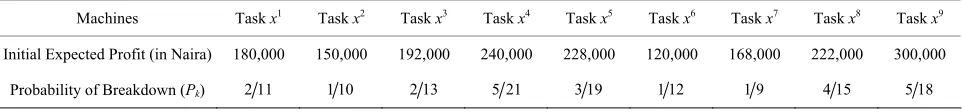
A production company in Nigeria proposed to purc se 50 machines that can perform nine different tasks. These

wn. The Table 2 gives

o maximize profit over T

ho

 



t1



ha

machines are subject to breakdo information of their decisions.

The company further estimated that out of the number of breakdown machines per week, 95% will join the functional ones for the next period.

The aim of the company is t rizon

Let st represents the number of machines to be

allo-cated in the next period, so that k

t t

s x s b . Since

s0

horizon,

f breakdown machines, and

is the number of machines at the beginning of the planning

1

m k k t k

P x





is the total number o

1 19 20

m

k t k

P x





e next period of operation, we have that

k

is expected to join the functional machines in th

1 1 20k

which is our transformation equ

1 m _, _, _{1, ,1}

k

t t k t

s s 



P x t T T   ,

ation and is a random variable.

We can now express our one-period expected return function as follows:

 

1

t t

x s b  (19)

, , 1, ,1

m

T T  .

 



1



0

k t t t

x s b 

 



 



 









Since the company cannot allocate negative resources

to any one task, we write , t = T, T –

1, ···, 1; k = 1, ···, m.

Of course, (19) is the same as

 

max

k

t t

s E_



T m tk



k





t

  



1 1

t

x_{X t}_ _k_

 

subject to

 



1



1

k

t t t

k

x s b s t



 



1 1 1

1

1 1

1

max

, 1, ,1,

max

1

, 20

k k

t

k k

t

m k

T t t t t t T t

x X k

m k

t t t t

x X k

m k

T t k t

k

F s x s b EF s

t T T

x s b

EF s P x



  

 

 

 

 



 

 _   _

 

 



 





 

 _  __

 





，

0 k t

x 

t = T, T – 1, ···, 1, and , t = T, T – 1, ···, 1; k = 1, ···,m.

Note: Our problem has 9 tasks and 48 periods.

Hence, m = 9 and T = 48. Set 1 9

  .

Therefore,

 



1 1 2 3 4

5 6 7 8

9

1 2 3 4

1 1

5 6 7

8 9

max 180000 150000 192000 240000

228000 120000 168000 222000

300000

1 2 1 2 5

20 11 10 13 21

3 1 1

13 12 9

4 5

15 18

1, 2, , k

T t

t t t t

x X

t t t t

t

T t t t t t

t t t

t t

F s

x x x x

x

F s x x x x

x x x

x x

T

 

 

   

   



 

 _    

 

  

  

  _

  48;t48, 47, ,1.

9

1 1

, 48, 47, ,1, k

t t

k

x S t



 





0 k

[image:6.595.58.539.681.737.2]

x 

Table 2. The Expected Initial Profit and Probability of Breakdown Machines.

Machines Task x1 _Task_x2_Task_x3_Task_x4_Task_x5 _Task_x6_Task_x7 _Task_x8_Task_x9 (20) subject to:

t , t = 48, 47, ···, 1; k = 1, ···, 9 which is a

paramet-ric linear programming problem with 9 variables.

A program using MatLab was used for (20). At the end, the following results were obtained.

The profit over 48 weeks is given by

Initial Expected Profit (in Naira) 180,000 150,000 192,000 240,000 228,000 120,000 168,000 222,000 300,000

(7)

 

48

F 0 91

1

4,571,1 0,000.

o

s  N s



By theorem 1.5, as T approach infinity, FT(s0)

ap-proaches F(s0),

422000 9

N

 422000 50

0

N 

 

0 0

lim T 409820000

T

lim

20, 491,000,000.

T T

F s F s

F s N s



 

N



 



and the al policy 9

 

0

t

optim x s , (t = 1, 2, ···), approaches

the lim

Discussion: Figure 1 shows the expected profit that

will accrued to the company over a period of 48 weeks. We found that at 48 weeks, the maximum profit that

it zero.

accrued to the company to be N4,571,100,000. Figure

[image:7.595.66.276.318.490.2]

2 shows the expected profit that will accrued to the

[image:7.595.70.275.528.700.2]

Figure 1. The Expected Profit that will accrued to the Company over a Period of 48 weeks.

Figure 2. The Expected Profit that will accrued to the Company over an Infinite Period.

an an e w It nd t

infinity, the maximum profit that will accrued to the an

comp y over infinit eeks. was fou that a

comp y to be N20, 491,0

6. Conclusion

Many production companies have for long been allocating resources to different tasks without putting into con-sideration certain factors that may hinder the realization of their objectives. This paper dealt with allocation of machines to tasks in order to maximize profit over finite and infinite horizon. Careful analysis of the situation reveals that adequate planning, prompt and effective maintainance can enhances the profitability of the com-pany.

REFERENCES

[1] J. M. Mulvey and H. Vladimirou, “Stochastic Network Programming for Financial Planning Problems,” Manage-

00,000.

ment Science, Vol. 38, No. 11, 1992, pp. 1642-1664. doi:10.1287/mnsc.38.11.1642

[2] B. Van Roy, D. P. Bertsekas, Y. Lee and J. N. Tsitsiklis, “A Neuro-Dynamic Programming Approach to Retailer

Inventory M the 36th IEEE

Conference

anagement,” Proceedings of

on Decision and Control, San Diego, 10-12 , pp. 4052-4057.

C.1997.652501 December 1997

doi:10.1109/CD

gramming, Elsevier, Amsterdam, 2003, pp. 555-635. [5] W. B. Powell, “Approximate Dynamic Programming for

Asset Manag versity, Princeton,

2004.

6. rogramming Algorithm for [3] W. B. Powell, “A Comparative Review of Alternative

Algorithms for the Dynamic Vehicle Allocation Prob- lem,” In: B. Golden and A. Assad, Eds., Vehicle Routing: Methods and Studies, North Holland, Amsterdam, 1988, pp. 249-292.

[4] W. B. Powell and H. Topaloglu, “Stochastic Program- ming in Transportation and Logistics,” In: A. Ruszczyn- ski and A. Shapiro, Eds., Handbook in Operation Re- search and Management Science, Volume on Stochastic Pro

ement,” Princeton Uni

[6] H. Topaloglu and S. Kunnumkal, “Approximate Dynamic Programming Methods for an Inventory Allocation Prob-lem under Uncertainty,” Cornell University, Ithaca, 200 [7] C. I. Nkeki, “On A Dynamic P

Resource Allocation Problems,” Unpublished M.Sc. The-sis, University of Ibadan, Ibadan, 2006.