Heuristic sequence selection for inventory routing problem

Authors are encouraged to submit new papers to INFORMS journals by means of a style file template, which includes the journal title. However, use of a template does not certify that the paper has been accepted for publication in the named jour-nal. INFORMS journal templates are for the exclusive purpose of submitting to an INFORMS journal and should not be used to distribute the papers in print or online or to submit the papers to another publication.

Heuristic Sequence Selection for

Inventory Routing Problem

Ahmed Kheiri

Lancaster University Management School, Department of Management Science,

Lancaster, LA1 4YX, UK.

[email protected]

In this paper, an improved sequence-based selection hyper-heuristic method for the Air Liquide inventory routing problem, the subject of the ROADEF/EURO 2016 challenge, is described. The organisers of the challenge have proposed a real-world problem of inventory routing as a difficult combinatorial optimisation problem. An exact method often fails to find a feasible solution to such problems. On the other hand, heuris-tics may be able to find a good quality solution that is significantly better than those produced by an expert human planner. There is a growing interest towards self configuring automated general-purpose reusable

heuristic approaches for combinatorial optimisation. Hyper-heuristics have emerged as such methodologies. This paper investigates a new breed of hyper-heuristics based on the principles of sequence analysis to solve the inventory routing problem. The primary point of this work is that it shows the usefulness of the improved sequence-based selection hyper-heuristic, and in particular demonstrates the advantages of using a data science technique of hidden Markov model for the heuristic selection.

Key words: Hyper-heuristic; Data Science; Inventory Routing; Scheduling; Healthcare

1.

Introduction

Many innovative and powerful search methods are tailored for their specific applications to underpin

effective search methodologies. On the other hand, hyper-heuristics are a set of techniques that

operate on (and explore) the space of heuristics as opposed to directly searching the space of

solutions (Burke et al. 2013). There goal is to raise the level of generality by offering search

methodologies to solve a wide range of optimisation problems instead of single problem domain.

Broadly, hyper-heuristics split into one of two classes: They can be used toselect between existing

heuristics (e.g. mutation operations or hill climbers) orgeneratenew heuristics to aid in solving hard

computational problems. This work focuses on the selection hyper-heuristics which are motivated

by the reasoning that the online learning of different combinations of low level heuristics will

yield improved algorithmic performance, and the goal is to discover the optimal (or near-optimal)

combinations of low level heuristics. The reader is directed to (Burke et al. 2013) for a recent survey

of hyper-heuristics.

Traditionally, a single-point-based search selection hyper-heuristic framework (in which search is

performed using a single complete candidate solution) utilises two consecutive methods: aselection

methodto select a suitable low level heuristic from a suite of heuristics and apply it to a candidate

solution, and a move acceptance method which decides whether to accept or reject the newly

generated solution. The method proposed in this work extends the first component of the traditional

selection hyper-heuristic framework to choose a sequence of low level heuristics and apply them

consecutively to a candidate solution as if a single operator.

Several empirical studies have shown that the choice of the selection hyper-heuristic components

and their parameter settings may significantly impact the overall performance of the hyper-heuristic

not only across different problem domains but also across different instances within the same

domain (Kheiri and ¨Ozcan 2016, Bilgin, ¨Ozcan, and Korkmaz 2007). A wide range of recent methods

attempt to remedy this by allowing machine learning and statistical techniques, ‘data science’,

so that hyper-heuristic itself can learn to configure, tune, adapt and so optimise better (Parkes, ¨

Ozcan, and Karapetyan 2015). This interaction between hyper-heuristic and data science promotes

more accurate prediction and better control of the decisions that hyper-heuristic algorithms make

during their execution. A wide range of data science techniques have been studied in the literature

and employed to effectively and automatically configure or design adaptive hyper-heuristic search

algorithms, utilising either online or offline knowledge extracted. This interaction has been made

by allowing data science methods to access the details of the optimisation process but in a

problem-domain independent manner. Examples of such methods include reinforcement learning in heuristic

selection ( ¨Ozcan et al. 2010), Taguchi method for parameters tuning (G¨um¨u¸s, ¨Ozcan, and Atkin

2016), genetic programming for heuristic selection (Nguyen, Zhang, and Johnston 2011), hidden

Markov model for heuristic sequence selection (Kheiri and Keedwell 2017, Wilson et al. 2018,

Ahmed, Mumford, and Kheiri 2019) and tensor-based approach for improved hyper-heuristic (Asta

and ¨Ozcan 2015, Asta, ¨Ozcan, and Curtois 2016).

It is always of interest to researchers and practitioners to detect the cutting-edge method

for solving a given problem and competitions play an important role in this pursuit. The

ROADEF/EURO Challenge 2016 (http://challenge.roadef.org/2016/en) proposed a

real-world problem of inventory routing with a focus on healthcare services delivering large volumes

of liquid oxygen to large numbers of hospitals worldwide, whilst observing a variety of constraints

(https://www.airliquide.com/). The goal is to assign delivery and loading shifts to match the

demand requirements subject to a set of soft and hard constraints taking into account pickups, time

windows, orders, drivers’ safety regulations and more in order to minimise the total distribution

cost and maximise the total quantity delivered over the planning horizon.

Although, the ultimate goal of hyper-heuristic research is to raise the level of generality by

offering a solution method that has the ability to work on a wide range of problem domains; still

it would be interesting to know the position of hyper-heuristics with respect to other methods

in a given problem domain while still being general. In this work, an improved sequence-based

selection hyper-heuristic utilising a data science technique as a competing method is proposed as

an easy-to-implement, yet effective approach to tackle this scheduling and routing problem. We

extend the solution model proposed in (Kheiri and Keedwell 2015, Kheiri et al. 2015) to allow the

hyper-heuristic to control the application of the selected sequence of heuristics to a particular part

of the solution.

With minimal tuning and problem specific expertise, the performance of the proposed

hyper-heuristic solver is significantly better than the other competing approaches, producing the best

solutions across all of the released problem instances.

The paper is structured as follows: In Section 2 we describe the tackled problem, and in Section 3

we introduce our proposed improved sequence-based selection hyper-heuristic method. Section 4

presents the empirical results. Finally, Section 5 concludes the study.

2.

Inventory Routing Problem

Due to the extreme difficulties in inventory routing problem (IRP), this area of study appeals to

strong interest of many researchers and practitioners. The problem dates back to 1980s (Bell et al.

1983). The main difference between inventory routing problems and classical vehicle routing

prob-lems is that the vendor coordinates the inventories of the customers, forecasting each customer’s

future consumption over the coming hours and days; and deciding how much and when inventories

should be replenished by routing vehicles. In logistics, this policy is called Vendor Management

Inventory (VMI). We also distinguish another set of customers referred to as ‘call-in’ customers,

which are supplied on an on-demandpolicy. A solution to the inventory routing is defined as a set

of routes visiting customers and delivering a specified amount of product at each of these sites in

order to maintain satisfactory inventory levels at all customers. In addition to routing constraints,

the orders of the call-in customers must be satisfied within specified time windows, the safety and

regulatory constraints (for example, limits on maximal driving time) must be respected, and the

run-outs must be avoided (i.e. the quantity of product stored at each customer site must not be

have to be satisfied such as consideration that drivers’basesand sourcesof product are not always

co-located, assignment of drivers to trailers are not pre-decided, shifts compose of several trips

that can alternate loading from source sites and deliveries to customer sites, and finally we assume

accurate modelling of time (continuous time for the timing of operations and discrete time for

inventory control).

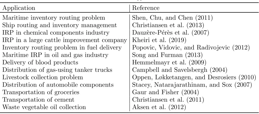
Table 1 presents some selected applications of the inventory routing problems.

Table 1 Some selected applications of the IRP

Application Reference

Maritime inventory routing problem Shen, Chu, and Chen (2011)

Ship routing and inventory management Christiansen et al. (2013) IRP in chemical components industry Dauz`ere-P´er`es et al. (2007) IRP in a large cattle improvement company Kheiri et al. (2019)

Inventory routing problem in fuel delivery Popovic, Vidovic, and Radivojevic (2012) Maritime IRP in oil and gas industry Song and Furman (2013)

Delivery of blood products Hemmelmayr et al. (2009)

Distribution of gas-using tanker trucks Campbell and Savelsbergh (2004)

Livestock collection problem Oppen, Løkketangen, and Desrosiers (2010)

Distribution of automobile components Stacey, Natarajarathinam, and Sox (2007)

Transportation of groceries Gaur and Fisher (2004)

Transportation of cement Christiansen et al. (2011)

Waste vegetable oil collection Aksen et al. (2012)

Some exact approaches, such as branch and cut algorithm (Archetti et al. 2007, Solyalı and

S¨ural 2011, Coelho and Laporte 2013b, Adulyasak, Cordeau, and Jans 2014, Coelho and Laporte

2013a), have been used by researchers to solve the IRP. However, due to the N P-hard nature of

the problem, metaheuristics are preferred in most of the previous studies. Metaheuristic algorithms

used in this problem include local search (Bertazzi, Paletta, and Speranza 2002, Benoist et al.

2011), greedy randomised adaptive search procedure (GRASP) (Dubedout et al. 2012), adaptive

large neighbourhood search (Coelho, Cordeau, and Laporte 2012b,a), tabu search (Archetti et al.

2012), ant colony optimisation algorithm (Huang and Lin 2010), memetic algorithm (Boudia and

Prins 2009), genetic algorithm (Abdelmaguid and Dessouky 2006), variable neighbourhood search

(Zhao, Chen, and Zang 2008), heuristic column generation algorithm (Michel and Vanderbeck

2012) and other algorithms (Savelsbergh and Song 2008, Bertazzi, Paletta, and Speranza 2005,

Raa and Aghezzaf 2009). To the best of our knowledge, the use of hyper-heuristic methods for the

inventory routing problem domain remains unexplored in the scientific literature.

Several variants of the IRP have been studied, including: IRP with a single customer (Solyalı

and S¨ural 2008), IRP with multiple customers (Chien, Balakrishnan, and Wong 1989), IRP with

and Speranza 2008), multi-item IRP (Sindhuchao et al. 2005), IRP with multiple suppliers (Benoist

et al. 2011), IRP with heterogeneous fleet (Persson and G¨othe-Lundgren 2005), stochastic inventory

routing problem (SIRP) at which customer demands are estimated probabilistically (Bard et al.

1998), SIRP with a finite horizon (Liu and Lee 2011), SIRP with an infinite horizon (Kleywegt,

Nori, and Savelsbergh 2002), dynamic IRP at which customer demand is gradually revealed over

time (Berbeglia, Cordeau, and Laporte 2010), dynamic SIRP at which customer demand is known

in a probabilistic fashion and revealed over time (Coelho, Cordeau, and Laporte 2014a), among

others. For the recent survey on inventory routing problem the reader is directed to (Coelho,

Cordeau, and Laporte 2014b, Archetti and Speranza 2016).

2.1. Problem Setting

The detailed description of the problem studied in this work can be found on the competition

website and in (Benoist et al. 2011); however, for completeness we summarise it in this section.

A solution to the studied multi-depot inventory routing problem is defined as a set of shifts, each

defined by the base (location from which it starts and ends), the resources (combination of a driver

and a trailer), the starting and ending dates, and the chronologically-ordered list of operations. An

operation is defined by the site (customer site or source site) where the operation takes place, the

quantity delivered (if customer site) or loaded (if source site), its arrival date, and its departure

date. Finally, a layover is defined as the fixed idle time interval in a shift that has one or more

layover customers, which enables the driver to drive for an extended duration in order to cover a

larger area. Over twenty constraintsare expected to be satisfied:

• C01 Layover duration: any travel between two sites that lasts more than a predefined

layover duration plus driving time are considered as layover.

• C02 Layover customers:if there is a visit to one or more layover customers, then the shift

must include a layover.

• C03 Maximum layover: only one layover per shift is allowed.

• C04 Shift constraint:each shift can be assigned to only one driver and only one trailer.

• C05 Base site:a driver has to start from the base and return back to the base.

• C06 Inter-shifts duration: two consecutive shifts assigned to the same driver must be

separated by a predefined duration.

• C07 Maximal driving duration:cumulated driving time per shift must not exceed a

pre-defined value.

• C08 Drivers’ time windows:the starting and ending dates for each shift must fit in one of

the time windows of the selected driver.

• C10 Allowable driver/trailer combinations: the assigned trailer in a shift must be one

of the trailers that can be driven by the driver.

• C11 Tank capacity: the tank capacity for each site must be respected.

• C12 Travelling time:arrival at a site requires travelling time from previous site, and

even-tually the layover duration.

• C13 Loading and delivery: loading and delivery operations take a predefined setup time

• C14 Deliveries’ time windows:the arrival and departure dates for each delivery must fit

in one of the opening times of the customer site.

• C15 Allowable trailer/customer combinations:delivery operations require the customer

site to be accessible for the selected trailer.

• C16 Allowable trailer/source combinations: loading operations require the source site

to be accessible for the selected trailer.

• C17 Trailer capacity:the sum of delivered amounts on any visit must not exceed the vehicle

capacity.

• C18 Initial quantity:initial quantity of a trailer for a shift is the end quantity of the trailer

following the previous shift.

• C19 VMI customer site capacity: the delivered quantity of a VMI customer must not

exceed the customer tank capacity.

• C20 Minimum deliverable amount: the delivered quantity of a VMI customer must be

greater than the minimum operation quantity for that customer.

• C21 Call-in customer: no delivery if there is no order.

• C22 Call-in customers satisfaction:each order should be satisfied by at least one operation

that should begin after the earliest time and before the latest time of the order. Note that the

model could create multiple deliveries to satisfy the total amount delivered requirement.

• C23 Call-in customer site capacity:the delivered quantity of a call-in customer must not

exceed the ordered quantity.

• C24 Call-in customer site quantity: ‘order quantity flexibility’ can be defined as the

minimum ratio of the ordered quantity to deliver to a call-in customer in order to consider the

order as satisfied.

• C25 Run-out avoidance:for each VMI customer, the tank level must be maintained at a

level greater than or equal to a certain safety level at all times.

The economic function to minimise is the cost per delivered unit over the long term:

P

∀s∈shif tsCost(s)

The cost of a shift includes: distance cost (total length of the shift, related to the trailer used),

time cost (total duration of the shift, related to the driver), and layover cost (if the shift contains

a layover).

3.

Methodology

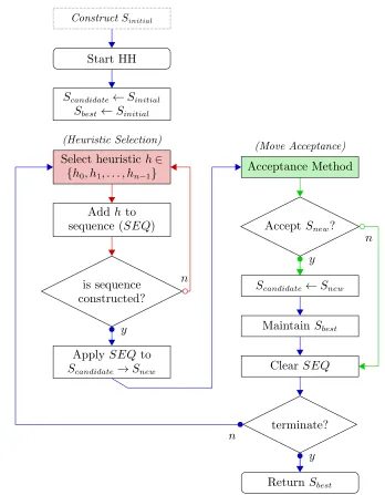
Figure 1 illustrates how a sequence-based selection hyper-heuristic framework operates. A notable

difference from a standard selection hyper-heuristic framework is that the excessive application of

single heuristics could cause the search process to get stuck at local optima. In contrast, applying

sequences of heuristics may lead the search to potentially jump from local optima, but might have

a net worsening of the objective, however, then such worsening moves are subject to the move

acceptance component to decide whether to accept or reject them.

The method applied in this work uses the generic sequence-based selection hyper-heuristic

frame-work as a basis, aiming to analyse and produce sequences of heuristics during an optimisation

using a hidden Markov model (HMM) (Baum and Petrie 1966) (see Algorithm 1), where hidden

states are replaced with low level heuristics. To accomplish this, we distinguish two matrices: a

transition score matrix (TM atrix[ ][ ]) to determine the movement between these states and another

score matrix (ASM atrix[ ][ ]) to determine whether the selected sequence will be applied to a

cur-rent solution (AS= 1) or will be coupled with another low level heuristic to form a sequence of heuristics (AS= 0). Assuming the following set of low level heuristics H={h0, h1, . . . , hn−1}, all

HMM matrices are initially assigned to 1. Whenever a sequence of heuristics improved the quality

of the best solution in hand, the relevant HMM scores get updated and increased by 1.

Conse-quently, during the optimisation the sequence-based hyper-heuristic adapts itself to detect a list of

‘promising’ sequences of heuristics that perform well. At any given step, the probability of moving

from hi tohj is given by the following formula:

Tmatrix[hi][hj] P

∀k(Tmatrix[hi][hk])

(2)

The probability of selecting the acceptance strategyl of hi is given by:

ASmatrix[hi][l] P

∀k(ASmatrix[hi][k])

(3)

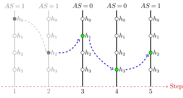
Figure 2 provides an example of four low level heuristics to illustrate how this method works.

Assume that h2 is invoked and that we are at step 3. Now based on the roulette wheel selection

method given the HMM matrices, the next low level heuristich1 is chosen withAS= 0; therefore,

h1 is added to the recordSEQ. Heuristich3withAS= 0 is selected next, hence,h3is added to the

growing sequence of heuristicsSEQ. We move to the next step where h2 is selected with AS= 1.

ConstructSinitial

Start HH

Scandidate←Sinitial

Sbest ←Sinitial

Select heuristich∈ {h0, h1, . . . , hn−1}

Addh to sequence (SEQ)

is sequence constructed?

Apply SEQto

Scandidate→Snew

Acceptance Method

AcceptSnew?

Scandidate←Snew

MaintainSbest

Clear SEQ

terminate?

ReturnSbest

(Heuristic Selection)

(Move Acceptance)

y

y

y n

n

n

Figure 1 A generic sequence-based selection hyper-heuristic framework

(SEQ={h1, h3, h2}) and will be applied toScandidateto return a new solutionSnew. Assuming that

Snew is better than the best solution in hand, then all the relevant scores are increased by one

as a reward, increasing the chance of selecting the sequence that generates improved solutions. In

this example, the following scores will be increased:Tmatrix[h2][h1], Tmatrix[h1][h3], Tmatrix[h3][h2],

ASmatrix[h1][0], ASmatrix[h3][0] andASmatrix[h2][1].

3.1. Overall Solution Model

Previous works (see for example (Dubedout et al. 2012)) define two-phase approaches, where the

first phase aims to construct an initial solution, followed by an improvement phase where the

Algorithm 1 SSHH Utilising Hidden Markov Model

1: LetH={h0, h1, . . . , hn−1} represent the set of heuristics; 2: LetTM atrix[hk][hl] represent the score of moving fromhk tohl;

3: LetASM atrix[hk][l] represent the score of applying acceptance strategyl forhk;

4: LetSbest, Scandidate, Snew represent the best, candidate and new solution, respectively;

5: LetSEQ represent the vector of a data-type that has three variables hprevious, hcurrent, AS;

6: fori←0,1, . . . , n−1 do

7: forj←0,1, . . . , n−1 do

8: TM atrix[hi][hj] = 1;

9: fori←0,1, . . . , n−1 do

10: forj←0,1do

11: ASM atrix[hi][j] = 1;

12: Scandidate, Snew, Sbest←ConstructSolution();

13: hcurrent←SelectRandom(H);

14: while timeLimitNotExceeded do

15: hprevious←hcurrent;

16: hcurrent←RouletteWheel(TM atrix, hprevious);

17: AS←RouletteWheel(ASM atrix, hcurrent);

18: SEQ.Add(hprevious, hcurrent, AS);

19: if AS= 1 then

20: Snew←Scandidate;

21: foreach iin SEQ do

22: Snew←Apply(i.hcurrent, Snew);

23: if Accept(Scandidate, Snew) then

24: Scandidate←Snew;

25: if Snew isBetterThanSbest then

26: Sbest←Snew;

27: foreach iin SEQ do

28: TM atrix[i.hprevious][i.hcurrent] =TM atrix[i.hprevious][i.hcurrent] + 1;

29: ASM atrix[i.hcurrent][i.AS] =ASM atrix[i.hcurrent][i.AS] + 1;

30: SEQ.Clear();

Step 1

AS= 1

h3

h2

h1

h0

2

AS= 1

h3

h2

h1

h0

3

AS= 0

h3

h2

h1

h0

4

AS= 0

h3

h2

h1

h0

5

AS= 1

h3

h2

h1

h0

Figure 2 An example to illustrate how the method works

phase and starts with an empty solution. A candidate solution is evaluated in terms of hard

constraint violations (i.e. feasibility) and logistic ratio. However, a weight is used to balance the

optimisation between the logistic ratio (which is equal to the time and distance cost divided by the

total quantity delivered over the whole horizon) and the violations of hard constraints. The value

of the weight has been determined manually here to ensure that hard constraint violation is highly

penalised. This implies that hard constraints are not considered strictly hard but are simply much

more heavily penalised than the logistic ratio. The hard constraints are the number of customer

orders that were not met and the time spent by customers with an inventory below their safety

level.

A solution is encoded as a set of routes (shifts), each defines a driver, a trailer and a set of

sites to visit. To evaluate a given solution, it has to be converted into a direct representation by

invoking two consecutive methods; the first to schedule the timing to their earliest possible time

while respecting all the hard constraints defined in Section 2.1, and the second method to decide

on the quantities of the product to be delivered or loaded. In the latter method, if the current site

is a customer, then we assign the least possible amount of product to deliver; otherwise if the site

is a source, then all the remaining quantities will be given to the previous customer sites, starting

from the nearest ones.

The sequence selection method is parameter-free; but there is a threshold parameter to set for

the move acceptance method. A generated solution is accepted by the move acceptance method

if either its quality is better than or equal to the quality of the candidate solution (quality(new

solution)≤quality(current solution)), or its quality is better than the quality of the best solution

in hand plus a threshold value (quality(new solution) < quality(best solution) +T×quality(best solution)). The value of the parameterT is calculated as follows:

T=

0.001 if best solution is not feasible

0.0001 + 0.01∗(1−telapsed/tlimit) otherwise.

where telapsed is the time elapsed in seconds, andtlimit is the total time limit in seconds.

3.2. Low Level Heuristics

The sequence-based selection hyper-heuristic (SSHH) method mixes a set of nineteen fairly simple

low level domain-specific heuristics.

• LLH0:Insert a new customer site into a selected route. However, if the best recorded solution

in hand is not feasible, then this heuristic lists all the demands and orders and inserts the customer

site with the earliest unsatisfied demand or order into a randomly selected route.

• LLH1: Insert a new source site into a selected route.

• LLH2: Change the location of the layover (if exists) in a selected route.

• LLH3: Reverse a block of sites in a selected route.

• LLH4: Delete a site from a selected route.

• LLH5: Replace a site with a new customer site in a selected route. However, if the best

recorded solution in hand is not feasible, then this heuristic lists all the demands and orders and

replaces a randomly selected site with the customer site that has the earliest unsatisfied demand

or order.

• LLH6: Replace a site with a new source site in a selected route.

• LLH7:Delete a site from a selected route, and re-insert it in a different location in the same

selected route.

• LLH8: Same as LLH7 but inserting a block of sites.

• LLH9: Swap two sites in a selected route.

• LLH10:Swap two blocks of sites in a selected route.

• LLH11:Change the trailer in a selected route.

• LLH12: Select a site from a random router1 and a site from another random router2 and

swap.

• LLH13:Same as LLH12 but swapping a block of sites.

• LLH14:Delete a site from a selected route, and insert it in a different location in a different

route.

• LLH15:Same as LLH14 but deleting and inserting a block of sites.

• LLH16:Merge a selected route with another route.

• LLH17:Swap two trailers of two selected routes.

• LLH18:Swap two drivers of two selected routes.

What distinguishes the proposed method in this work from the original sequence-based selection

hyper-heuristic proposed in (Kheiri and Keedwell 2015) is that each low level heuristic is associated

previously modified routes during the application of a given sequence (S = 0); or a randomly selected route (S= 1). As an example, if the hyper-heuristic selected the following sequence to apply LLH1-LLH0-LLH4, and the selected solution parameters were (1-0-1); then LLH1 will insert

a new source site into a random route (r1), followed by applying LLH0 which will insert a new

customer site into the same route (r1), followed by applying LLH4 which will delete a site from

a randomly selected route (r2). We let the SSHH to adaptively learn the solution parameter by

introducing a new HMM matrix.

4.

Results

In ROADEF/EURO Challenge 2016, three problem sets denoted by A, B and X were created to

test the competitors’ solvers. The first two sets were public to the competitors while X instances

were hidden.

Initially, eleven instances (set-A) were released for the qualification phase and the participants

(41 teams) were invited to submit their solvers and solutions to those instances at the end of the

phase. The organisers compared the performance of the submitted solvers running them under the

time limit of 30 minutes of multi-threaded execution for each A instance on a standard machine.

The qualified teams (12 teams) were announced continuing to the final phase, when a second set

of 15 instances (set-B) was released. Similarly, at the end of this phase, the finalists were invited

to submit their solvers and solutions to the B instances. Then the organisers ran those solvers on

the set-B instances and another set of five hidden instances (set-X) to determine the winner of

the challenge. The hidden X instances were released after the end of the challenge. The solvers

submitted by the finalists (9 teams) were tested on the 20 instances of subsets B and X. A single

run for each instance, each for 30 minutes was conducted. The final objective values obtained

from each solver for each instance were ranked to determine the winner of the ROADEF/EURO

Challenge 2016.

The ranking of the solvers was determined as follows. Let O(I, T) be the final objective value obtained by teamT for instanceI. LetObest(I) be the best objective value over instanceI obtained

among all participants. Then:

score(I, T) = 1−e

Obest(I)−O(I,T)

Obest(I) ₍₅₎

S17 S15 S18 S24 S12 J09 S26 S25 S09 S23 S13 J08 0.0

1.0 2.0 3.0 4.0 5.0 6.0 7.0 8.0

SSHH

Team

Score

Set-A Instances

Figure 3 Results of the qualification phase

S17 S15 S24 S12 J09 S13 S09 S23 S25 0.0

2.0 4.0 6.0 8.0 10.0 12.0 14.0

SSHH

Team

Score

Set-B Instances

S17 S15 S24 S12 J09 S13 S09 0.0

5.0 10.0 15.0 20.0

SSHH

Team

Score

Set-B and Set-X Instances

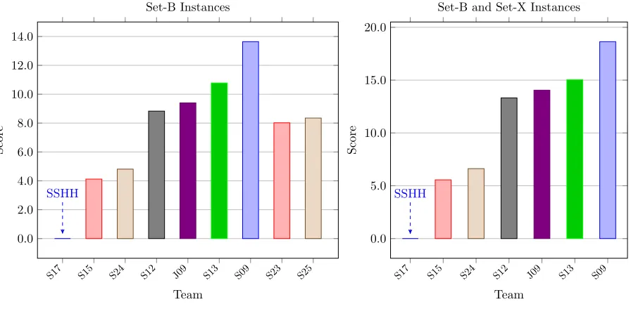
Figure 4 Results of the final phase

The team ranking results of the qualification phase and the final phase are provided in Figures 3

and 4, respectively.

Our approach (Team S17) outperformed all the other algorithms and produced the best solution

for all instances in both qualification and final phases. This provides indication that the employment

of a data science technique, which was a deliberate decision on our part, gives a robust solver

evidenced by the performance obtained on the hidden instances which were not available at the

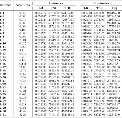
Table 2 Summary of experimental results. Feasibility: time required to obtain feasible solution (in seconds),

LR: logistic ratio, TSC: total shifts cost and TDQ: total delivered quantity.

Instance Feasibility 3 minutes 30 minutes LR TSC TDQ LR TSC TDQ

A-1 0.055 0.055177 53738.00 973917.00 0.055021 53562.00 973486.00 A-2 0.066 0.055095 53752.00 975617.00 0.054792 53266.00 972147.00 A-3 0.016 0.023124 2933.950 126879.80 0.022954 2973.660 129549.03 A-4 0.000 0.027470 5811.920 211573.03 0.027105 5811.510 214403.95 A-5 0.000 0.015523 2772.800 178623.20 0.015320 2720.000 177550.13 A-6 0.109 0.017589 10596.75 602481.18 0.016263 10136.85 623315.77 A-7 0.063 0.016522 10152.95 614510.51 0.015768 9685.070 614224.58 A-8 0.000 0.010136 1557.400 153648.80 0.010009 1961.340 195964.54 A-9 2.901 0.021280 36619.56 1720883.2 0.017888 31609.95 1767136.1 A-10 0.015 0.024782 5462.200 220412.37 0.025606 5232.800 204361.58 A-11 1.560 0.040436 27980.26 691960.37 0.035028 24317.46 694233.48 B-12 3.713 0.011694 25837.18 2209472.7 0.010266 22398.88 2181947.3 B-13 0.016 0.032089 8404.000 261898.09 0.030768 8313.300 270192.58 B-14 1.778 0.042855 32947.40 768808.33 0.037582 28449.90 757005.96 B-15 0.140 0.027111 7069.300 260755.18 0.026608 7067.360 265613.55 B-16 0.141 0.013155 8065.690 613140.93 0.012420 7800.430 628047.87 B-17 11.06 0.037834 32545.05 860214.53 0.031538 26934.65 854030.68 B-18 15.74 0.038122 31432.76 824522.29 0.033018 27510.50 833208.31 B-19 0.562 0.041304 31038.70 751465.68 0.036018 26467.70 734838.07 B-20 16.52 0.021855 45192.10 2067811.7 0.018656 37635.23 2017275.4 B-21 7.035 0.020729 41013.86 1978562.3 0.017210 34639.86 2012811.8 B-22 70.18 0.016487 75630.12 4587371.8 0.012992 59681.85 4593776.1 B-23 82.48 0.016356 74752.79 4570465.6 0.013311 62221.93 4674428.9 B-24 0.031 0.013385 8282.370 618777.28 0.013033 8016.330 615067.04 B-25 0.265 0.013985 16607.44 1187475.8 0.012411 14652.95 1180611.1 B-26 0.437 0.013982 16572.10 1185208.1 0.012866 15324.29 1191049.2 X-27 3.572 0.012048 26500.80 2199529.1 0.010234 22504.99 2199123.3 X-28 0.218 0.013240 7793.830 588650.43 0.012410 7286.530 587140.47 X-29 9.984 0.039053 32903.80 842548.09 0.031905 27435.56 859927.47 X-30 40.42 0.015907 72462.23 4555300.1 0.013015 61765.63 4745719.2 X-31 82.24 0.016385 74131.95 4524483.1 0.013994 64727.03 4625451.6

4.1. An Analysis of SSHH

The experiments have been performed on an i3-2120 CPU at 3.30GHz with 8GB RAM. A

multi-thread independent search implementation of the proposed sequence-based selection hyper-heuristic

is employed, at which each concurrent thread executes the same sequence-based selection

hyper-heuristic method and they do not communicate during the search process, only at the end to

identify the best overall solution. Each thread will almost certainly explore different regions of the

solution space and return different solutions. Table 2 summaries the results.

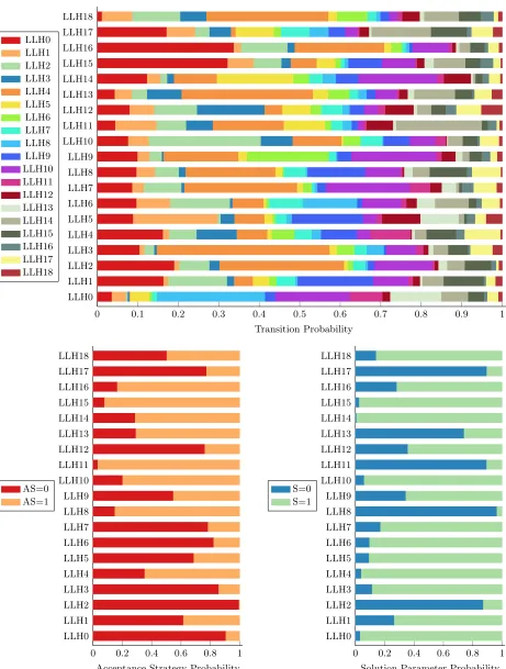
Figure 5 provides the scores (probabilities) of the transition and associated sequence-based

accep-tance strategy and solution parameter matrices of each low level heuristic while solving an arbitrary

instance (B-12) for 3 minutes. The HMM matrices show that several heuristics are being invoked

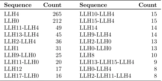
Table 3 The top 20 constructed sequences of low level heuristics while solving instance B-12

Sequence Count Sequence Count

LLH4 265 LLH10-LLH4 15

LLH0 212 LLH15-LLH4 15

LLH11-LLH4 49 LLH14 14

LLH13-LLH4 45 LLH9-LLH4 14

LLH2-LLH4 36 LLH2-LLH0 13

LLH1 31 LLH0-LLH0 13

LLH9-LLH0 25 LLH8 10

LLH11-LLH0 20 LLH13-LLH15-LLH4 9

LLH12 17 LLH0-LLH4 8

LLH17-LLH0 16 LLH2-LLH11-LLH4 8

best solutions in hand for the same instance are reported in Table 3. Although single heuristics are

frequently used, the approach clearly identifies sequences of size 2 and 3 as useful to the search.

LLH4, which deletes a site from a given route, is involved in most of these sequences, an interesting

finding.

5.

Conclusion

Hyper-heuristics are high level search methodologies and can be broadly classified into selection

hyper-heuristics, also known as ‘heuristics to choose heuristics’, or generation hyper-heuristics

(Burke et al. 2013). The solution method used in this work is based on the selection type of

hyper-heuristics that controls a set of pre-defined low level hyper-heuristics under an iterative framework. The

proposed approach aims to exploit several low level heuristics, each LLH attempts to enhance an

aspect of the quality of the current solution during the optimisation process. Traditionally, selection

hyper-heuristics identify two main consecutive stages, aselection stageto select a suitable heuristic

and apply it to the candidate solution, and a move acceptance stage to decide whether to accept

or reject the newly generated solution. The sequence-based selection hyper-heuristic replaces the

first stage of the traditional selection hyper-heuristic framework in order to select sequences of

heuristics instead of a single heuristic. These are then applied sequentially to the current solution.

The proposed method has been successfully applied to an inventory routing problem, a subject of

the ROADEF/EURO 2016 challenge, and the results demonstrate the effectiveness of the method,

being the winner of the challenge against 41 teams across 16 different countries, producing the best

solutions across all of the released problem instances.

As for the future work, although the heuristic selection mechanism of the improved

sequence-based selection hyper-heuristic is parameter-free, the move acceptance component introduces a

single parameter that is currently tuned after some experimentation. We plan to work on a learning

strategy to adapt the parameter value during the search process. Similar to the work in (Asta

et al. 2016), we also intend to hybridise genetic algorithms with sequence-based hyper-heuristics

0 0.1 0.2 0.3 0.4 0.5 0.6 0.7 0.8 0.9 1 LLH0 LLH1 LLH2 LLH3 LLH4 LLH5 LLH6 LLH7 LLH8 LLH9 LLH10 LLH11 LLH12 LLH13 LLH14 LLH15 LLH16 LLH17 LLH18 Transition Probability LLH0 LLH1 LLH2 LLH3 LLH4 LLH5 LLH6 LLH7 LLH8 LLH9 LLH10 LLH11 LLH12 LLH13 LLH14 LLH15 LLH16 LLH17 LLH18

0 0.2 0.4 0.6 0.8 1 LLH0 LLH1 LLH2 LLH3 LLH4 LLH5 LLH6 LLH7 LLH8 LLH9 LLH10 LLH11 LLH12 LLH13 LLH14 LLH15 LLH16 LLH17 LLH18

Acceptance Strategy Probability AS=0

AS=1

0 0.2 0.4 0.6 0.8 1 LLH0 LLH1 LLH2 LLH3 LLH4 LLH5 LLH6 LLH7 LLH8 LLH9 LLH10 LLH11 LLH12 LLH13 LLH14 LLH15 LLH16 LLH17 LLH18

Solution Parameter Probability S=0

S=1

References

Abdelmaguid TF, Dessouky MM, 2006A genetic algorithm approach to the integrated inventory-distribution problem. International Journal of Production Research 44(21):4445–4464.

Adulyasak Y, Cordeau JF, Jans R, 2014 Formulations and branch-and-cut algorithms for multivehicle pro-duction and inventory routing problems.INFORMS Journal on Computing 26(1):103–120.

Ahmed L, Mumford C, Kheiri A, 2019 Solving urban transit route design problem using selection hyper-heuristics.European Journal of Operational Research 274(2):545–559.

Aksen D, Kaya O, Salman FS, Ak¸ca Y, 2012 Selective and periodic inventory routing problem for waste vegetable oil collection.Optimization Letters 6(6):1063–1080.

Archetti C, Bertazzi L, Hertz A, Speranza MG, 2012 A hybrid heuristic for an inventory routing problem.

INFORMS Journal on Computing 24(1):101–116.

Archetti C, Bertazzi L, Laporte G, Speranza MG, 2007A branch-and-cut algorithm for a vendor-managed inventory-routing problem. Transportation Science41(3):382–391.

Archetti C, Speranza MG, 2016The inventory routing problem: the value of integration.International Trans-actions in Operational Research 23(3):393–407.

Asta S, Karapetyan D, Kheiri A, ¨Ozcan E, Parkes AJ, 2016 Combining Monte-Carlo and hyper-heuristic methods for the multi-mode resource-constrained multi-project scheduling problem.Information Sciences

373:476–498.

Asta S, ¨Ozcan E, 2015A tensor-based selection hyper-heuristic for cross-domain heuristic search.Information Sciences 299:412–432.

Asta S, ¨Ozcan E, Curtois T, 2016 A tensor based hyper-heuristic for nurse rostering. Knowledge-Based Systems 98:185–199.

Bard JF, Huang L, Jaillet P, Dror M, 1998A decomposition approach to the inventory routing problem with satellite facilities.Transportation Science 32(2):189–203.

Baum LE, Petrie T, 1966Statistical inference for probabilistic functions of finite state Markov chains. The Annals of Mathematical Statistics 37(6):1554–1563.

Bell WJ, Dalberto LM, Fisher ML, Greenfield AJ, Jaikumar R, Kedia P, Mack RG, Prutzman PJ, 1983

Improving the distribution of industrial gases with an on-line computerized routing and scheduling

optimizer.Interfaces 13(6):4–23.

Benoist T, Gardi F, Jeanjean A, Estellon B, 2011 Randomized local search for real-life inventory routing.

Transportation Science 45(3):381–398.

Berbeglia G, Cordeau JF, Laporte G, 2010 Dynamic pickup and delivery problems. European Journal of Operational Research 202(1):8–15.

Bertazzi L, Paletta G, Speranza MG, 2005 Minimizing the total cost in an integrated vendor—managed

inventory system.Journal of Heuristics 11(5):393–419.

Bertazzi L, Savelsbergh M, Speranza MG, 2008Inventory Routing, 49–72 (Boston, MA: Springer US).

Bilgin B, ¨Ozcan E, Korkmaz EE, 2007An experimental study on hyper-heuristics and exam scheduling. Burke EK, Rudov´a H, eds.,Practice and Theory of Automated Timetabling VI, volume 3867 ofLecture Notes

in Computer Science, 394–412 (Springer Berlin Heidelberg).

Boudia M, Prins C, 2009 A memetic algorithm with dynamic population management for an integrated production-distribution problem.European Journal of Operational Research 195(3):703–715.

Burke EK, Gendreau M, Hyde M, Kendall G, Ochoa G, ¨Ozcan E, Qu R, 2013Hyper-heuristics: a survey of

the state of the art.Journal of the Operational Research Society 64(12):1695–1724.

Campbell AM, Savelsbergh MWP, 2004A decomposition approach for the inventory-routing problem. Trans-portation Science 38(4):488–502.

Chien TW, Balakrishnan A, Wong RT, 1989An integrated inventory allocation and vehicle routing problem.

Transportation Science 23(2):67–76.

Christiansen M, Fagerholt K, Flatberg T, Haugen O, Kloster O, Lund EH, 2011Maritime inventory

rout-ing with multiple products: A case study from the cement industry. European Journal of Operational

Research 208(1):86–94.

Christiansen M, Fagerholt K, Nygreen B, Ronen D, 2013Ship routing and scheduling in the new millennium.

European Journal of Operational Research 228(3):467–483.

Coelho LC, Cordeau JF, Laporte G, 2012aConsistency in multi-vehicle inventory-routing. Transportation

Research Part C: Emerging Technologies 24:270–287.

Coelho LC, Cordeau JF, Laporte G, 2012b The inventory-routing problem with transshipment. Computers

& Operations Research 39(11):2537–2548.

Coelho LC, Cordeau JF, Laporte G, 2014aHeuristics for dynamic and stochastic inventory-routing.

Com-puters & Operations Research 52:55–67.

Coelho LC, Cordeau JF, Laporte G, 2014bThirty years of inventory routing.Transportation Science48(1):1–

19.

Coelho LC, Laporte G, 2013a A branch-and-cut algorithm for the multi-product multi-vehicle inventory-routing problem.International Journal of Production Research 51(23-24):7156–7169.

Coelho LC, Laporte G, 2013bThe exact solution of several classes of inventory-routing problems.Computers

& Operations Research 40(2):558–565.

Dauz`ere-P´er`es S, Nordli A, Olstad A, Haugen K, Koester U, Per Olav M, Teistklub G, Reistad A, 2007

Omya hustadmarmor optimizes its supply chain for delivering calcium carbonate slurry to european

Dubedout H, Dejax P, Neagu N, Yeung TG, 2012A GRASP for real life inventory routing problem:

appli-cation to bulk gas distribution.9th International Conference on Modeling, Optimization & SIMulation

(Bordeaux, France), URLhttps://hal.archives-ouvertes.fr/hal-00728664.

Gaur V, Fisher ML, 2004A periodic inventory routing problem at a supermarket chain.Operations Research

52(6):813–822.

G¨um¨u¸s DB, ¨Ozcan E, Atkin J, 2016 An Analysis of the Taguchi Method for Tuning a Memetic Algorithm

with Reduced Computational Time Budget, 12–20 (Cham: Springer International Publishing).

Hemmelmayr V, Doerner KF, Hartl RF, Savelsbergh MWP, 2009 Delivery strategies for blood products

supplies.OR Spectrum 31(4):707–725.

Huang SH, Lin PC, 2010A modified ant colony optimization algorithm for multi-item inventory routing

prob-lems with demand uncertainty.Transportation Research Part E: Logistics and Transportation Review

46(5):598–611.

Kheiri A, Dragomir AG, Mueller D, Gromicho J, Jagtenberg C, van Hoorn JJ, 2019Tackling a vrp challenge

to redistribute scarce equipment within time windows using metaheuristic algorithms. EURO Journal

on Transportation and Logistics URLhttp://dx.doi.org/10.1007/s13676-019-00143-8.

Kheiri A, Keedwell E, 2015 A sequence-based selection hyper-heuristic utilising a hidden Markov model.

Proceedings of the 2015 on Genetic and Evolutionary Computation Conference, 417–424, GECCO ’15.

Kheiri A, Keedwell E, 2017A hidden Markov model approach to the problem of heuristic selection in

hyper-heuristics with a case study in high school timetabling problems.Evolutionary Computation 25(3):473–

501.

Kheiri A, Keedwell E, Gibson MJ, Savic D, 2015Sequence analysis-based hyper-heuristics for water

distribu-tion network optimisadistribu-tion.Procedia Engineering119:1269–1277, Computing and Control for the Water

Industry (CCWI2015) Sharing the best practice in water management.

Kheiri A, ¨Ozcan E, 2016An iterated multi-stage selection hyper-heuristic.European Journal of Operational

Research 250(1):77–90.

Kleywegt AJ, Nori VS, Savelsbergh MWP, 2002The stochastic inventory routing problem with direct

deliv-eries.Transportation Science 36(1):94–118.

Liu SC, Lee WT, 2011 A heuristic method for the inventory routing problem with time windows. Expert

Systems with Applications 38(10):13223–13231.

Michel S, Vanderbeck F, 2012 A column-generation based tactical planning method for inventory routing.

Operations Research 60(2):382–397.

Nguyen S, Zhang M, Johnston M, 2011A genetic programming based hyper-heuristic approach for

combina-torial optimisation. Proceedings of the 13th Annual Conference on Genetic and Evolutionary

Oppen J, Løkketangen A, Desrosiers J, 2010 Solving a rich vehicle routing and inventory problem using

column generation.Computers & Operations Research 37(7):1308–1317.

¨

Ozcan E, Misir M, Ochoa G, Burke EK, 2010 A reinforcement learning - great-deluge hyper-heuristic for

examination timetabling.International Journal of Applied Metaheuristic Computing 1(1):39–59.

Parkes AJ, ¨Ozcan E, Karapetyan D, 2015A Software Interface for Supporting the Application of Data Science

to Optimisation, 306–311 (Cham: Springer International Publishing).

Persson JA, G¨othe-Lundgren M, 2005Shipment planning at oil refineries using column generation and valid

inequalities. European Journal of Operational Research 163(3):631–652.

Popovic D, Vidovic M, Radivojevic G, 2012Variable neighborhood search heuristic for the inventory routing

problem in fuel delivery.Expert Systems with Applications 39(18):13390–13398.

Raa B, Aghezzaf EH, 2009A practical solution approach for the cyclic inventory routing problem.European

Journal of Operational Research 192(2):429–441.

Savelsbergh M, Song JH, 2008An optimization algorithm for the inventory routing problem with continuous

moves.Computers & Operations Research 35(7):2266–2282.

Shen Q, Chu F, Chen H, 2011A lagrangian relaxation approach for a multi-mode inventory routing problem

with transshipment in crude oil transportation.Computers & Chemical Engineering 35(10):2113–2123.

Sindhuchao S, Romeijn HE, Ak¸cali E, Boondiskulchok R, 2005 An integrated inventory-routing system for

multi-item joint replenishment with limited vehicle capacity.Journal of Global Optimization 32(1):93– 118.

Solyalı O, S¨ural H, 2008 A single suppliersingle retailer system with an order-up-to level inventory policy.

Operations Research Letters 36(5):543–546.

Solyalı O, S¨ural H, 2011A branch-and-cut algorithm using a strong formulation and an a priori tour-based

heuristic for an inventory-routing problem.Transportation Science 45(3):335–345.

Song JH, Furman KC, 2013A maritime inventory routing problem: Practical approach.Computers &

Oper-ations Research 40(3):657–665.

Stacey J, Natarajarathinam M, Sox C, 2007 The storage constrained, inbound inventory routing problem.

International Journal of Physical Distribution & Logistics Management 37(6):484–500.

Wilson D, Rodrigues S, Segura C, Loshchilov I, Hutter F, Buenfil GL, Kheiri A, Keedwell E, Ocampo-Pineda

M, zcan E, Pea SIV, Goldman B, Rionda SB, Hernndez-Aguirre A, Veeramachaneni K, Cussat-Blanc S, 2018Evolutionary computation for wind farm layout optimization. Renewable Energy 126:681–691.

Zhao QH, Chen S, Zang CX, 2008 Model and algorithm for inventory/routing decision in a three-echelon