Optimizing Deep Learning Inference on Embedded Systems
Through Adaptive Model Selection
VICENT SANZ MARCO
∗,
FCRAL, Osaka University, JapanBEN TAYLOR
∗,
MetaLab, Lancaster University, United KingdomZHENG WANG,
University of Leeds, United KingdomYEHIA ELKHATIB,
MetaLab, Lancaster University, United KingdomDeep neural networks (DNNs) are becoming a key enabling technique for many application domains. However, on-device inference on battery-powered, resource-constrained embedding systems is often infeasible due to prohibitively long inferencing time and resource requirements of manyDNNs. Offloading computation into the cloud is often unacceptable due to privacy concerns, high latency, or the lack of connectivity. While compression algorithms often succeed in reducing inferencing times, they come at the cost of reduced accuracy. This paper presents a new, alternative approach to enable efficient execution ofDNNson embedded devices. Our approach dynamically determines whichDNNto use for a given input, by considering the desired accuracy and inference time. It employs machine learning to develop a low-cost predictive model to quickly select a pre-trainedDNNto use for a given input and the optimization constraint. We achieve this by first training off-line a predictive model, and then use the learnt model to select aDNNmodel to use for new, unseen inputs. We apply our approach to two representativeDNNdomains: image classification and machine translation. We evaluate our approach on a Jetson TX2 embedded deep learning platform, and consider a range of influential
DNNmodels including convolutional and recurrent neural networks. For image classification, we achieve a 1.8x reduction in inference time with a 7.52% improvement in accuracy, over the most-capable singleDNNmodel. For machine translation, we achieve a 1.34x reduction in inference time over the most-capable single model, with little impact on the quality of translation.
∗Both authors contributed equally to this research.
Conference Extension: A preliminary version of this article appeared in ACM LCTES 2018 [58]. The extended version makes the several additional contributions over the conference paper:
(1) A new case study has been added in the form of Neural Machine Translation (Section6), demonstrating adaptability; (2) It introduces a new, better approach for deep learning model selection (Section3.2); (3) It improves upon the Model Selection Algorithm, allowing different selection strategies (Section3.3); (4) It provides a performance breakdown of different selection strategies for the Model Selection Algorithm (Section7.2), providing new insights on the impact of algorithm selection strategies; (5) It includes an analysis of resource utilisation (Section7.6.2), showing how the choices of model selection affect resource footprints; (6) It presents new experimental results when combining our approach with compression (Section7.6.3), showing how model selection can be applied and combined with model compression techniques; (7) The Discussion has been updated to reflect the work added (Section8); (8) The Related Work has been updated to reflect recent work, and add work relevant to new contributions (Section9).
Authors’ addresses: Vicent Sanz Marco, FCRAL, Osaka University, Japan, [email protected]; Ben Taylor, MetaLab, Lancaster University, United Kingdom, [email protected]; Zheng Wang, University of Leeds, United Kingdom, [email protected]; Yehia Elkhatib, MetaLab, Lancaster University, United Kingdom.
Permission to make digital or hard copies of all or part of this work for personal or classroom use is granted without fee provided that copies are not made or distributed for profit or commercial advantage and that copies bear this notice and the full citation on the first page. Copyrights for components of this work owned by others than ACM must be honored. Abstracting with credit is permitted. To copy otherwise, or republish, to post on servers or to redistribute to lists, requires prior specific permission and/or a fee. Request permissions from [email protected].
© 2019 Association for Computing Machinery. XXXX-XXXX/2019/11-ART $15.00
ACM Reference Format:
Vicent Sanz Marco, Ben Taylor, Zheng Wang, and Yehia Elkhatib. 2019. Optimizing Deep Learning Inference on Embedded Systems Through Adaptive Model Selection. 1, 1 (November 2019),26pages.https://doi.org/10. 475/123_4
1 INTRODUCTION
Deep learning is getting a lot of attention recently, and with good reason. It has proven ability
in solving many difficult problems such as object recognition [10,21], facial recognition [42,56],
speech processing [2], and machine translation [3]. While many of these tasks are also important
application domains for embedded systems [33], existing deep learning solutions are often resource
intensive tasks, consuming a considerable amount of CPU, GPU, memory, and power [6]. Without
optimization, we are left with a disparity between the resources required and the resources available, leading to long inferencing times, and making real-time applications infeasible on battery-powered, resource-limited embedded devices.
Numerous optimization tactics have been proposed to enable deep inference1on embedded
devices. Prior approaches are either architecture specific [53], or come with drawbacks. Model
compression is a commonly used technique for acceleratingDNNson embedded devices. Using
compression, aDNNcan be optimised by reducing its resource and computational requirements [14,
18,19,23]. Unfortunately, this also comes at a cost, a reduction in model accuracy. To avoid this,
alternate approaches have been developed; offload some, or all, computation to a cloud server where
the resources are available for fast inference times [28,59]. This, however, is not always possible. A
fast, reliable network is not always guaranteed, leading to high latency [11]. Furthermore, sending
sensitive data over a network could be prohibited due to privacy constraints.
Our work seeks to offer an alternative to execute pre-trainedDNNmodels on embedded systems.
Our aim is to design ageneralizableapproach to optimiseDNNsto runefficient, embeddedinference
without affecting accuracy. Central to our approach is the design of an adaptive scheme to determine, at runtime, which of the availableDNNsis the best fit for the input and evaluation criterion. Our key insight is that the optimal model – the model which is able to give the correct input in the fastest
time – depends on the input data and the evaluation criterion. In fact, by utilising multipleDNN
models we are able to increase accuracy in some cases. In essence, for a simple input – an image taken under good lighting conditions, with a contrasting background; or a short sentence with little punctuation – a simple, fast model would be sufficient; a more complex input would require a more complex model. Similarly, if an accurate output with high confidence is required a more sophisticated but slower model would have to be employed – otherwise, a simple model would be good enough. Given the diverse and evolving nature of user requirements, applications workloads,
andDNNmodels themselves, the best model selection strategy is likely to change over time. This
ever-evolving nature makes automatic heuristic design highly attractive – heuristics can be easily updated to adapt to the changing application context.
To achieve our goals, we employ machine learning (ML) toautomaticallyconstruct a predictor
able to dynamically select the optimum model to use. Our predictor is first trainedoff-line. Then,
using a set of automatically tuned features of theDNNinput, the predictor determines the optimum
DNNfor anew, unseeninput; taking into consideration the evaluation criterion. We show that
our approach can automatically derive high-quality heuristics for different evaluation criteria. The learned strategy can effectively leverage the prediction capability and runtime overhead of
candidateDNNs, leading to an overall better accuracy when compared with the most capableDNN
model, but with significantly less runtime overhead. Compression can be used in conjunction to
1Inference in this work means applying a pre-trained model on an input to obtain the corresponding output. This is different
Optimizing Deep Learning Inference on Embedded Systems Through Adaptive Model Selection:3
M o b i l e n e t R e s N e t _ v 1 _ 5 0 I n c e p t i o n _ v 2R e s N e t _ v 2 _ 1 5 2 0 . 0
0 . 5 1 . 0 1 . 5 2 . 0
+
+
*
*
+
*
+ O p t i m a l t o p - 5 s c o r e m o d e l
In
fe
re
n
c
e
T
im
e
(
s
) I m a g e 1 I m a g e 2 I m a g e 3
O p t i m a l t o p - 1 s c o r e m o d e l
*
[image:3.486.50.422.86.156.2](a) Image 1 (b) Image 2 (c) Image 3 (d) Inference time
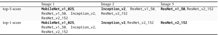
Fig. 1. The inference time (d) of four CNN-based image recognition models when processing images (a) - (c). The target object is highlighted on each image. This example (combined with Table1) shows that the optimal model (i.e.the fastest one that gives an accurate output) depends on the success criterion and the input.
Table 1. List of models that give the correct prediction per image under the top-5 and the top-1 scores.
Image 1 Image 2 Image 3
top-5 score MobileNet_v1_025,
ResNet_v1_50, Inception_v2, ResNet_v2_152
Inception_v2, ResNet_v1_50, ResNet_v2_152
ResNet_v1_50,ResNet_v2_152
top-1 score MobileNet_v1_025,
ResNet_v1_50, Inception_v2, ResNet_v2_152
Inception_v2,ResNet_v2_152 ResNet_v2_152
our approach to generate multipleDNNsof varying capability, then automatically choose the best
at runtime. This is a new way for optimizing deep inference on embedded devices.
Our approach is designed to be generally applicable to all domains of deep learning. As case studies, we choose two typical and unique domains for evaluation: image classification and
machine translation. Both domains have a dynamic range of availableDNNarchitectures including
convolutional and recurrent neural networks. We evaluate our approach on the NVIDIA Jetson
TX2 embedded platform and consider a wide range of influentialDNNmodels, ranging from simple
to complex. Experimental results show that our approach delivers portable good performance
across the twoDNNtasks. For image classification, it improves the inference accuracy by 7.52% over
the most-capable single DNN model while achieving 1.8x less inference time. For machine
translation, it reduces the inference time of 1.34x over the most-capable model with negligible impact on the quality of the translation.
The paper makes the following technical contributions:
• We present a novelMLbased approach to automatically learn how to selectDNNmodels based
on the input and precision requirement (Section3). Our system has little training overhead
as it does not require any modification to pre-trainedDNNmodels;
• Our work is the first to leverage multipleDNNmodels to improve the prediction accuracy and
reduce inference time on embedded systems (Section7).
• Our approach has a good generalization ability as it works effectively on different network
architectures, application domains and input datasets. We show that our approach can be easily integrated with existing model compression techniques to improve the overall results.
2 MOTIVATION
As a motivation, consider two contrasting examples, image classification and machine translation,
of usingDNNs. The experiments in this section are carried out on a NVIDIA Jetson TX2 platform
where we use the GPU for inference; full details of the system can be seen in Section4.1.
2.1 Image Classification
Setup. For image classification, we investigate one subset of DNNs: Convolutional Neural
[image:3.486.55.432.213.274.2]3 _ l a y e r g n m t _ 2 _ l a y e r g n m t _ 4 _ l a y e r g n m t _ 8 _ l a y e r
0
1 0 0 0 2 0 0 0 3 0 0 0 4 0 0 0 5 0 0 0
*
+
+
*
O p t i m a l B L E U - P S s c o r e m o d e l O p t i m a l B L E U s c o r e m o d e l
+
*
In
fe
re
n
c
e
T
im
e
(
m
s
)
S e n t e n c e 1 S e n t e n c e 2 S e n t e n c e 3
+
+
*
3 _ l a y e r g n m t _ 2 _ l a y e r g n m t _ 4 _ l a y e r g n m t _ 8 _ l a y e r
0
1 0 2 0 3 0 4 0 5 0
B
L
E
U
s
c
o
re
S e n t e n c e 1 S e n t e n c e 2 S e n t e n c e 3
[image:4.486.51.426.77.172.2](a) Runtime (b) BLEU scores
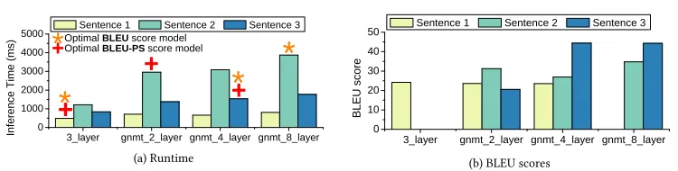
Fig. 2. The inference time, optimal model (a), and BLEU score (b) of three sentences (shown in Table2). Here the optimal model achieves the highest score for an evaluation criteria. Model names explained in footnote3.
Inception[25],ResNet[22], andMobileNet[23]2. Specifically, we used the following models:
MobileNet_v1_025, theMobileNetarchitecture with a width multiplier of 0.25;ResNet_v1_50,
the first version ofResNetwith 50 layers;Inception_v2, the second version of Inception; and
ResNet_v2_152, the second version ofResNetwith 152 layers. All these models are built upon
TensorFlow [1] and have been pre-trained by independent researchers using the ImageNet ILSVRC
2012training dataset[48].
Evaluation Criteria.Each model takes an image as input and returns a list of label confidence values as output. Each value indicates the confidence that a particular object is in the image. The resulting list of object values are sorted in descending order regarding their prediction confidence, so that the label with the highest confidence appears at the top of the list. In this example, the accuracy of a model is evaluated using the top-1 and the top-5 scores defined by the ImageNet Challenge. Specifically, for the top-1 score, we check if the top output label matches the ground truth label of the primary object; and for the top-5 score, we check if the ground truth label of the primary object is in the top 5 of the output labels for each given model.
Results.Figure1d shows the inference time per model using three images from the ImageNet
ILSVRCvalidation dataset. Recognizing the main object (a cottontail rabbit) from the image shown
in Figure1a is a straightforward task. We can see from Table1that all models give the correct answer
under the top-5 and top-1 score criterion. For this image,MobileNet_v1_025is the best model to use
under the top-5 score, because it has the fastest inference time – 6.13x faster thanResNet_v2_152.
Clearly, for this image,MobileNet_v1_025is good enough, and there is no need to use a more
advanced (and expensive) model for inference. If we consider a slightly more complex object
recognition task shown in Figure1b, we can see thatMobileNet_v1_025is unable to give a correct
answer regardless of our success criterion. In this caseInception_v2should be used, although this
is 3.24x slower thanMobileNet_v1_025. Finally, consider the image shown in Figure1c, intuitively
it can be seen that this is a more difficult image recognition task, as the main object is a similar color to the background. In this case the optimal model changes depending on our success criterion.
ResNet_v1_50is the best model to use under top-5 scoring, completing inference 2.06x faster than
ResNet_v2_152. However, if we use top-1 for scoring we must useResNet_v2_152to obtain the
correct label, despite it being the most expensive model. Inference time for this image is 2.98x
and 6.14x slower thanMobileNet_v1_025for top-5 and top-1 scoring respectively. The results are
similar if we use different images of similar complexity levels.
2Each model architecture follows its own naming convention.MobileNet_vi_j, whereiis the version number, andjis a
width multiplier out of 100, with 100 being the full uncompressed model.ResNet_vi_j, whereiis the version number, and
Optimizing Deep Learning Inference on Embedded Systems Through Adaptive Model Selection:5
Table 2. The sentences used in Figure2 Sentence ID Sentence
1 High on the agenda are plans for greater nuclear co-operation.
2 Advertisements, documentaries, TV series and parts in films consumed his next decade but after his 2008 BBC series, LennyHenry.tv, he thought: " What are you going to do next, Len, because it all feels a bit like you’re marking time or you’re slightly going sideways."
3 Kenya has started biometrically registering all civil servants in an attempt to remove "ghost workers" from the government’s payroll.
Input Feature
Extraction Inference Model
Selection Output
Fig. 3. Overview of our approach.
Y Model 1 Input
features Distance calculation Model 1? N
Model 2?
Model 2 N
Model n?
Model n N
KNN-1 KNN-2 KNN-n
all models will fail
...
Y Y
Fig. 4. Ourpremodelfor image classification, made up of a series
ofKNNmodels predicting whether to use a specificDNNor not. Our
process for selecting classifiers is described in Section3.3.
2.2 Machine Translation
Setup.In the second experiment, we consider the following 4 machine translation models as they
provide a range of accuracy and runtime capabilities3:3_layer,gnmt_2_layer,gnmt_4_layer, and
gnmt_8_layer. We chose three distinct sentences from the WMT15/16 English-German newstest
dataset [60], which can be seen in Table2.
Evaluation Criteria.Unlike image classification, no metrics similar to top-1 and top-5 exist for machine translation. Therefore, we use the following metrics for evaluation:
• BLEU(higher is better). Bilingual Evaluation Understudy is widely used to evaluate machine translation model output. It returns a value between 0 and 1, 1 being a perfect output; it is very rarely achieved.
• BLEU-PS(higher is better). BLEU per second. BLEU is only able to represent a degree of correctness, we also use BLEU-PS to evaluate the trade-off between BLEU and inference time. BLEU-PS is similar to Energy Delay Product (EDP, which is used to evaluate the trade-off
between energy consumption and runtime), and is calculated as BLEUI nf er×.T imeBLEU.
Results.Figure2shows the inference time, BLEU score and optimal model for each sentence. Sentence 1, is the simplest sentence, therefore the easiest translation task. The optimal model for all
metrics is our simplest,3_layer. Surprisingly, our most complex model,gnmt_8_layer, fails on
this sentence; by using the cheapest model we achieve a higher accuracy 1.66x quicker. Similarly
the optimal model forSentence 3across both metrics isgnmt_4_layer. In this case, we cannot use
our cheapest model, as it fails. By choosing the optimal model forSentence 3we can infer 1.15x
quicker, without impacting accuracy. It is clear thatSentence 2is more complex thanSentence 1, it
is much longer, has frequent punctuation, and contains non-words,e.g.2008 and TV. In this case,
the optimal model changes depending on the evaluation metric. If we are optimising for BLEU-PS
we usegnmt_2_layer, which is 1.31x times quicker thangnmt_8_layer. However, if we would
like to maximise accuracy, we need to usegnmt_8_layer.
2.3 Summary of Motivation Experiments
3 OUR APPROACH 3.1 Overview
Figure3depicts the overall workflow of our approach. Our approach trades memory footprints for
accuracy and reduced inference time. At the core of our approach is a predictive model (termed
premodel) that takes anew, unseen input(e.g.an image or sentence), and predicts which of a set
of pre-trainedDNNmodels to use for that giveninput. This decision may vary depending on the
scoring method used at the time,e.g.either top-1 or top-5 in image classification.
Our premodelis automatically generated based on the problem domain. An example of a
generatedpremodelcan be seen in Figure4. The prediction of ourpremodelis based on a set of
quantifiable properties – orfeatures, such as the number of edges and brightness of an image – of
theinput. Once a model is chosen, theinputis passed to the selectedDNN, which then performs
inference on theinput. Finally, the inference output of the selectedDNNis returned. Use of our
premodelwill work in exactly the same way as any single modeli.e.the input and output will be
in the same format, however, we are able to dynamically select the best model to use.
3.2 Premodel Design
To design an effectivepremodelfor embedded inference, we consider two design goals: (i) high
accuracy and (ii) fast execution time. By correctly choosing the optimal model, a highly accurate
premodelcan reduce the average inference time. Furthermore, a fastpremodelis important because
if apremodeltakes much longer than any singleDNNwill be useless. The task of choosing a candidate
DNNto use is essentially a classification problem in machine learning. Although using a standardML
classifier as apremodelcan yield acceptable results, we discovered we can maximize performance
by changing thepremodelarchitecture depending on the domain (see Section3.3).
To construct a fast yet accuratepremodel, we consider a number of differentMLclassifiers.
Specifically, in this work we consider four well-established classifiers: K-Nearest Neighbour (KNN),
a simple clustering based classifier; Decision Tree (DT), a tree based classifier; Naive Bayes (NB), a
probabilistic classifier; and Support Vector Machine (SVM), a more complex, but well performing
classification algorithm. In Section7.1, we evaluate a number of differentMLtechniques, including
Decision Trees, Support Vector Machines, andCNNs.
Simultaneously, we consider two different types ofpremodelarchitecture: (i) A simple, single
classifier architecture using only oneMLclassifier to predict whichDNN to use; (ii) A multiple
classifier architecture (See Figure4), a sequence ofMLclassifiers where each classifier predicts
whether to use a singleDNNor not. The later is described in more detail in Section3.2.1. Finally, we
chose a set of features to represent eachinput; the selection process is detailed in in Section3.5.
3.2.1 Multiple Classifier Architecture. Figure4gives an overview of apremodelimplementing
a multiple classifier architecture. As an example, we will use the K-Nearest Neighbors (KNN) based
premodelcreated for image classification. For eachDNNmodel we wish to include in ourpremodel,
we use a separateKNNmodel. As ourKNNmodels are going to contain much of the same data, we
begin ourpremodelby calculating our K closest neighbours. Taking note of which record of training
data each of the neighbours corresponds to, we avoid recalculating the distance measurements;
instead, we simply change the labels of these data-points.KNN-1is the firstKNNmodel in our
premodel, through which all input to thepremodelwill pass.KNN-1predicts whether the input
image should useModel-1to classify it or not. IfKNN-1predicts thatModel-1should be used, then
thepremodelreturns this label, otherwise the features are passed on to the nextKNN,i.e. KNN-2.
This process repeats until the image reachesKNN-n, the finalKNNmodel in ourpremodel. In the
3We name our models using the following convention:{gnmt_}N_layer, we prefix the name withgnmt_where the model
Optimizing Deep Learning Inference on Embedded Systems Through Adaptive Model Selection:7
Algorithm 1Model Selection Require:data,θ, selection_method
1: Model_1_DN N=most_optimum_DN N(data)
2:cur r_DN N s.add(Model_1_DN N)
3:cur r_acc=дet_acc(cur r_DN N s)
4: acc_diff = 100 5: whileacc_diff>θdo
6: improvement_metric = next_selection_metric(selection_method)
7: next_DNN = greatest_improvement_DNN(data, curr_DNNs, improvement_metric) 8: cur r_DN N s.add(next_DN N)
9: new_acc=дet_acc(cur r_DN N s)
10: acc_diff = new_acc - curr_acc
11: cur r_acc=new_acc
12:end while
event thatKNN-npredicts that we should not useModel-n, the next step will depend on the user’s
declared preference: (i) use a pre-specified model, to receive some output to work with; or (ii) do not perform inference and inform the user of the failure.
3.3 Inference Model Selection
In Algorithm1we describe our selection process for choosing whichDNNs to include in our
premodel. This algorithm takes in three parameters: (1)data, containing the output of eachDNN
for everyinput; (2)θ, a threshold parameter telling us when to terminate the model selection
process; and (3)selection_method, one of a choice of methods that produces animprovement_metric
(accuracy or optimal) for determining when if a candiateDNNshould be included in thepremodel
in each iteration. We consider the following three model selection methods:
• Based on Accuracy.Using this selection method, we will add aDNNtopremodelif it has the greatest improvement in accuracy for each iteration. There are some cases where the selected
DNNsall fail to make a correct prediction, but some of the remaining candidate models can.
During each selection iteration, we will choose a remainingDNNthat if it is included, it can
lead to the most significant improvement in prediction accuracy forpremodel.
• Based on Optimal.In each iteration of the loop, the most optimalDNNis selected;i.e.the one that gives the greatest overall improvement in accuracy, but leads to the lowest increase
in inference time, for the selectedDNNset.
• Alternate.A hybrid of the first two approaches. We alternate between choosing the most
optimal and the most accurateDNNin each iteration. Our firstDNNis always the most optimal.
Model selection process.The model selection process works as follows.
• Initialization.The firstDNNwe include is the the most optimal model for our training data,
i.e., theDNNthat is most frequently considered to be optimal across training instances.
• Iterative selection.At each iteration, we consider each of the remaining potentialDNNs, and
add the one which brings the greatest improvement to ourimprovement_metric(accuracy or
optimal), which can change per iteration based on theselection_method.
• Termination.We iteratively add newDNNsuntil our accuracy improvement is lower than
the termination threshold,θ%.
Using this Model Selection Algorithm we are able to addDNNsthat best compliment one another
when working together, maximizing our accuracy while keeping our runtime low. In Section7.2
we evaluate the impact of different parameter choices on our algorithm.
Illustrative example.We now walk through the Model Selection Algorithm using the image
classification problem as an example. In this example, we set our thresholdθ to 0.5, which is
M .n e t _ v1 _
1 00 I n ce p
t i on _ v 1
R es n e t _v 1
_ 50 I n ce p
t i on _ v 2
R es n e t _v 2
_ 50 I n ce p
t i on _ v 3
R es n e t _v 1
_ 10 1 I n ce p
t i on _ v 4
R es n e t _v 2
_ 10 1
R es n e t _v 2
_ 15 2
R es n e t _v 1
_ 15 2
[image:8.486.260.431.95.138.2]0 2 0 4 0 6 0 8 0 % o f b e in g o p ti m a l
Fig. 5. How often aCNNmodel is considered to be
optimal under top-1 on the training dataset.
Training Data Inference Profiling Feature extraction optimum model feature values L ea rn in g A lg o rit h
m Predictive Model
Fig. 6. The training process. We use the same procedure to train each individual model within
thepremodelfor each evaluation criterion.
M .n e t _ v1 _
1 00 I n ce p
t . _v 1 I n ce p
t . _v 2 I n ce p
t . _v 4 R es n
e t _v 1 _ 50 R es n
e t _v 1 _ 10 1 R es n
e t _v 1 _ 15 2 R es n
e t _v 2 _ 50 R es n
e t _v 2 _ 10 1 R es n
e t _v 2 _ 15 2 0 . 0
0 . 4 0 . 8 1 . 2 1 . 6 2 . 0 2 . 4
In fe re n c e T im e ( s
) I n f e r e n c e t i m e
0
2 0 4 0 6 0 8 0 1 0 0 T o p - 1 a c c u r a c y
T o p -1 A c c u ra c y ( % )
I n ce p t i on _
v 1 I n ce p t i on _
v 2 I n ce p
t i on _ v 4
R es n e t _v 1
_ 50
R es n e t _v 1
_ 10 1
R es n e t _v 1
_ 15 2 R es n
e t _v 2 _ 50
R es n e t _v 2
_ 10 1
R es n e t _v 2
_ 15 2
0 1 0 2 0 3 0 4 0 5 0 T o p -1 A c c u ra c y ( % )
R es n e t _v 1
_ 50
R es n e t _v 1
_ 10 1
R es n e t _v 1
_ 15 2 R es n
e t _v 2 _ 50
R es n e t _v 2
_ 10 1
R es n e t _v 2
_ 15 2
0 5 1 0 1 5 2 0 2 5 T o p -1 A c c u ra c y ( % )
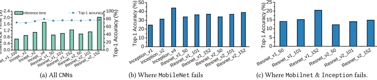
(a) AllCNNs (b) WhereMobileNetfails (c) WhereMobilnet&Inceptionfails.
Fig. 7. Image Classification – (a) The top-1 accuracy and inference time of allCNNswe consider. (b) The top-1
accuracy of allCNNson the images on whichMobileNet_v1_100fails. (c) The top-1 accuracy of allCNNson
the images on whichMobileNet_v1_100andInception_v4fails.
accuracy" for this example.We carry out a a sensitivity analysis for these parameters later in Section7.2.
Figure5shows the percentage of our training data that considers each of ourCNNsto be optimal.
For this example, the model selection process works as follows:
• First model.The first model is the most optimal model. In this example,MobileNet_v1_100
is chosen to beModel-1because it is optimal for most (70.75%) of our training data.
• Iterative selection.If we were to follow the “based on optimal" selection method and choose
the next most optimalCNN, we would chooseInception_v1. However, we do not do this
as it would result in ourpremodelbeing formulated of many cheap, yet inaccurate models.
Instead we choose to look at the training data and consider which of our remainingCNNs
gives the greatest improvement in accuracy (i.e., “based on accuracy"), as ’Accuracy’ is our
improvement_metric. Intuitively, as image classification is either right or wrong, we are
searching for theCNNthat is able to correctly classify the most of the remaining 29.25%
cases whereMobileNet_v1_100fails. As seen in Figure7b,Inception_v4is best, correctly
classifying 43.91% of the remaining data and creating a 12.84% increase inpremodelaccuracy;
leaving 16.41% of our data failing. Repeating this process (Figure7c), we addResNet_v1_152
to ourpremodel, further increasing total accuracy by 2.55%.
• Termination.After addingResNet_v1_152, we iterate once more to achieve apremodel
accuracy increase of less than 0.5% (θ), and therefore terminate.
• Results.After running this process, ourpremodelis composed of:MobileNet_v1_100for Model-1,Inception_v4forModel-2, andResNet_v1_152forModel-3.
3.4 Training the Premodel
Training ourpremodelfollows the standard procedure, and is a multi-step process. We describe
the entire training process in detail below, and provide a summary in Figure6. Generally, we need
to figure out which candidateDNNis optimum for each of our traininginputs(to be used by the
Model Selection Algorithm described in Section3.3), we then train ourpremodelto predict the
[image:8.486.57.438.194.275.2]Optimizing Deep Learning Inference on Embedded Systems Through Adaptive Model Selection:9
Generate Training Data.Our training dataset consists of the feature values and the corresponding
optimumDNNfor eachinputunder an evaluation criterion. To evaluate the performance of the
candidateDNN models, they must be applied to unseeninputs. We exhaustively execute each
candidateDNNon theinputs, measuring the inference time and prediction results. Inference time
is measured on an unloaded machine to reduce noise; it is a one-off cost –i.e.it only needs to be
completed once. Because the relative runtime of models is stable, training can be performed on a
high-performance server to speedup data generation. It is to note that adding a newDNNsimply
requires executing allinputson the newDNNwhile taking the same measurements described above.
Using the execution time, andDNNoutput results, we can calculate theoptimumclassifier for each
input;i.e.the model that achieves the accuracy goal (top-1, top-5, or BLEU) in the least amount of
time. Finally, we extract the feature values (described in Section3.5) from eachinput, and pair the
feature values to the optimum classifier for eachinput, resulting in our complete training dataset.
Building the Premodel.The training data is used to determine the classification models to use
and their optimal hyper-parameters. All classifiers we consider forpremodelsupport are supervised
learning algorithms. Therefore, we simply supply the classifier with the training data and it carries
out its internal algorithm. For example, inKNNclassification the training data is used to give a label
to each point in the model, then during prediction the model will use a distance measure (in our case we use Euclidian distance) to find the K nearest points (in our case K=5). The label with the highest number of points to the prediction point is the output label.
Training Cost.Total training time of ourpremodelis dominated by generating the training data, which took less than a day using a NVIDIA P40 GPU on a multi-core server. This can vary depending on the number of candidate inference models to be included. In our case, we had an unusually long
training time as we considered a large number ofDNNmodels. We would expect in deployment
that the user has a much smaller search space for potentialDNNs. The time in model selection and
parameter tuning is negligible (less than 2 hours) in comparison. See also Section7.4.
3.5 Features
One key aspect in building a successful predictor is selecting the right features to characterize the input. In this work, we have developed an automatic feature selection process, the user is simply required to provide a number of candidate features. Automatic feature generation could be used to provide candidate features, however this is out of the scope of this work.
3.5.1 Feature Selection. Feature extraction is the biggest overhead of ourpremodel, therefore
by reducing our feature count we can decrease the total execution time. Moreover, by reducing the
number of features we are also improving the generalizability of ourpremodel.
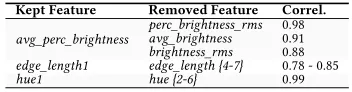
Initially, we use correlation-based feature selection. If pairwise correlation is high for any pair of features, we drop one of them and keep the other; retaining most of the information. We perform this by constructing a matrix of correlation coefficients using Pearson product-moment correlation
(PCC). The coefficient value falls between−1 and+1. The closer the absolute value is to 1, the
stronger the correlation between the two features being tested. We set a threshold of 0.75 and
removed any features that had an absolutePCChigher than the threshold.
Next, we evaluated the importance of each of our remaining features. To do so, we first trained
and evaluated ourpremodelusing K-Fold cross validation (see also Section7.4) and all of our
current features, recordingpremodelaccuracy. We then remove each feature and re-evaluate
the model on the remaining features, taking note of the change in accuracy. If there is a large drop in accuracy then the feature must be important, otherwise, the feature does not hold much importance for our purposes. Using this information we performed a greedy search, removing the
have summarized the result of each feature selection stage on both of our case studies. Removing any of the remaining features resulted in a significant drop in model accuracy.
3.5.2 Feature Scaling.The final step before passing our features to aMLmodel is scaling each
feature to a common range (between 0 and 1) in order to prevent the range of any single feature being a factor in its importance. Scaling does not affect the distribution or variance of feature values. To achieve this during deployment, we record the minimum and maximum values of each feature in the training dataset and use these to scale the corresponding features of new data.
3.6 Runtime Deployment
Deployment of our proposed method is designed to be simple and easy to use, similar to current
DNNusage techniques. We have encapsulated all of the inner workings, such as needing to read
the output of thepremodeland then choosing the correctDNNmodel. A user would interact with
ourpremodelby simply calling a prediction function and getting a result in return in the same
format as theDNNsin use. Using image classification as an example, the return value would be the
predicted labels and their confidence levels.
4 EVALUATION SETUP
We apply our approach to two representativeDNN domains: image classification and machine
translation. Each domain is presented as a case study (Sections5and6) which shows the results at
each stage of applying our approach; providing an end-to-end analysis. The case studies will end
with an analysis in Section7of how our approach performed against other representativeDNNsin
the domain. In the remaining of this section, we describe our evaluation setup and methodology.
4.1 Hardware and Software
Hardware.We evaluate our approach on the NVIDIA Jetson TX2 embedded deep learning platform. The system has a 64 bit dual-core Denver2 and a 64 bit quad-core ARM Cortex-A57 running at 2.0 Ghz, and a 256-core NVIDIA Pascal GPU running at 1.3 Ghz. The board has 8 GB of LPDDR4 RAM and 96 GB of storage (32 GB eMMC plus 64 GB SD card).
System Software.Our evaluation platform runs Ubuntu 16.04 with Linux kernel v4.4.15. We use
Tensorflow v.1.0.1, cuDNN (v6.0) and CUDA (v8.0.64). Ourpremodelis implemented using the
Python scikit-learn package. Our feature extractor is built upon OpenCV and SimpleCV.
4.2 Evaluation Methodology
4.2.1 Model Evaluation.We use 10-fold cross-validation to evaluate each premodel on its
respective dataset. Specifically, we split our dataset into 10 sets which equally represent the full
dataset,e.g.if we consider image classification, we partition the 50K validation images into 10
equal sets, each containing 5K images. We retain one set for testing our premodel, and the
remaining 9 sets are used as training data. We repeat this process 10 times (folds), with each of the 10 sets used exactly once as the testing data. This standard methodology evaluates the generalization ability of a machine-learning model.
We evaluate our approach using the following metrics:
• Inference time(lower is better). Wall clock time between a model taking in an input and
producing an output, including the overhead of ourpremodel.
• Energy consumption(lower is better). The energy used by a model for inference. For our
approach, this also includes the energy consumption of thepremodel. We deduct the static
power when the system is idle.
Optimizing Deep Learning Inference on Embedded Systems Through Adaptive Model Selection:11
Table 3. All features considered for image classification.
Feature Description
n_keypoints # of keypoints avg_brightness Average brightness
brightness_rms Root mean square of brightness avg_perc_brightness Average of perceived brightness perc_brightness_rms Root mean square of perceived brightness contrast The level of contrast
[image:11.486.262.438.110.156.2]edge_length{1-7} A 7-bin histogram of edge lengths edge_angle{1-7} A 7-bin histogram of edge angles area_by_perim Area / perimeter of the main object aspect_ratio The aspect ratio of the main object hue{1-7} A 7-bin histogram of the different hues
Table 4. Correlation values (absolute) of removed features to the kept ones for image classification.
Kept Feature Removed Feature Correl. perc_brightness_rms 0.98 avg_brightness 0.91 avg_perc_brightness
brightness_rms 0.88 edge_length1 edge_length {4-7} 0.78 - 0.85
hue1 hue {2-6} 0.99
Metrics for image classification.The following metrics are specific to image classification:
• Precision(higher is better). The ratio of a correctly predicted images to the total number
of images that are predicted to have a specific object. This metric answers e.g., “Of all the
images that are labeled to have a cat, how many actually have a cat?".
• Recall(higher is better). The ratio of correctly predicted images to the total number of test
images that belong to an object class. This metric answers e.g., “Of all the test images that
have a cat, how many are actually labeled to have a cat?".
• F1 score (higher is better). The weighted average of Precision and Recall, calculated as 2×RecallRecall×+Pr ecisionPr ecision. It is useful when the test datasets have an uneven distribution of classes.
Metrics for machine translation.The following metrics are specific to machine translation:
• BLEU(higher is better). Similar to precision in image classification. It is a measure of how
much the words (and/or n-grams) in theDNNmodel output appeared in the reference output(s).
• Rouge(higher is better). Similar to recall in image classification. It is a measure of how much
the words (and/or n-grams) in the reference output(s) appear in theDNNmodel output.
• F1 measure(higher is better). Similar to F1 score for image classification. The weighted
average of BLEU and Rouge, calculated as 2×RouдeRouдe×+BLEUBLEU.
4.2.2 Performance Report.We report thegeometric meanof the aforementioned evaluation
metrics across the cross-validation folds. To collect inference time and energy consumption, we run each model on each input repeatedly until the 95% confidence bound per model per input is
smaller than 5%. In the experiments, we exclude the loading time of theDNNmodels as they only
need to be loaded once in practice. However, we include the overhead of ourpremodelin all our
experimental data. To measure energy consumption, we developed a lightweight runtime to take readings from the onboard energy sensors at a frequency of 1,000 samples per second. It is to note that our work does not directly optimise for energy consumption. We found that in our scenario there is little difference when optimizing for energy consumption compared to time.
5 CASE STUDY 1: IMAGE CLASSIFICATION
To evaluate our approach in the domain of image classification we consider 14 pre-trainedCNN
models from the TensorFlow-Slim library [52]. The models are built using TensorFlow and trained
on the ImageNet ILSVRC 2012training set. We use the Imagenet ILSVRC 2012validation setto
create the training data for ourpremodel, and evaluate it usingcross-validation(see Section4.2).
5.1 Premodel for Image Classification
5.1.1 Feature Selection.In this work, we considered a total of 29 candidate features, shown
in Table3. The features were chosen based on previous image classification work [20],e.g.edge
based features (more edges lead to a more complex image), as well as intuition based on our
M .n et _ v 1 _1 00
I n ce p t i o n_ v 4
R es n e t _ v1 _
1 52 O ur s
0
1
2
3
In
fe
re
n
c
e
T
im
e
(
s
) i n f e r . m o d e l P r e m o d e l
M .n e t _ v1 _
1 00 I n ce p
t i o n_ v 4 R es n e
t _ v1 _ 1 52 O ur s
0
1
2
3
4
5 I n f e r . m o d e l P r e m o d e l
J
o
u
le
s
M .n et _ v 1 _1 0
0
I n ce p t i o n_ v 4 R es n e
t _ v1 _
1 52 O ur s O ra c l
e
4 0 6 0 8 0 1 0 0
A
c
c
u
ra
c
y
(
%
)
T o p - 1 T o p - 5
M .n et _ v 1 _1 00
I n ce p t i o n_ v 4
R es n e t _ v1 _
1 52 O ur s 0 . 0
0 . 2 0 . 4 0 . 6 0 . 8
1 . 0 P r e c i s i o n R e c a l l F 1
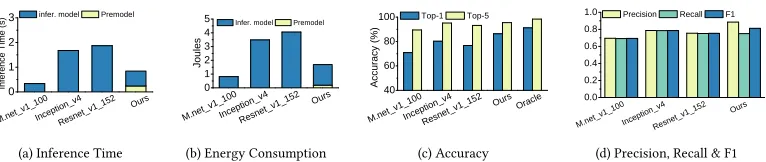
[image:12.486.57.440.82.163.2](a) Inference Time (b) Energy Consumption (c) Accuracy (d) Precision, Recall & F1
Fig. 8. Image Classification – Overall performance of our approach against individual models and anOracle
for inference time (a), energy consumption (b), accuracy (c), and precision, recall and F1 scores (d).
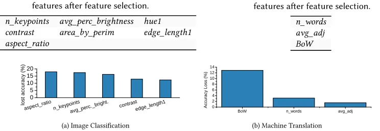
summarizes the features removed using correlation-based feature selection, leaving 17 features. Next, we iteratively evaluated feature importance and performed a greedy search that reduced our
feature count down to 7 features (see Table5). This process is described in Section3.5.1.
5.1.2 Feature Analysis.We now analyse the importance of each feature that was chosen during
our feature selection process. We calculate feature importance by first training apremodelusing
all of our chosen features (n), and note the accuracy of ourpremodel. In turn, we then remove each
feature, retraining and evaluating ourpremodelon the remainingn−1 features, noting the drop
in accuracy. We then normalize the values to produce a percentage of importance for each feature.
Figure9a shows the top 5 dominant features based on their impact on ourpremodelaccuracy. It is
clear our features hold a very similar level of importance, ranging between 18% and 11% for our most and least important feature respectively. The similarity of feature importance is an indication that each of our features is able to represent distinct information about each image. All of which is important for the prediction task at hand.
5.1.3 Creating The Premodel.Applying our automatic approach topremodelcreation, described
in Section3.2, resulted in implementing a multiple classifier architecture consisting of a series of
simpleKNNmodels. We found thatKNNhas a quick prediction time (<1ms) and achieves a high
accuracy for this problem. Furthermore, we applied our Model Selection Algorithm (Section3.3) to
determine whichCNNsto be included in thepremodel. As we have explained in Section3.3, this
process resulted in a choice of:MobileNet_v1_100forModel-1,Inception_v4forModel-2, and,
finally,ResNet_v1_152forModel-3. Finally, we use the training data generated in Section5.1.1and
10-fold-cross-validation to train and evaluate ourpremodel.
5.2 Overall Performance of Image Classification
5.2.1 Inference Time.Figure8a compares the inference time amongDNNmodels used by our
premodel and our approach. Due to space limitations we limit to these three models
(MobileNet_v1_100, Inception_v4, and ResNet_v1_152) since they are the ones used by our
premodel.MobileNet_v1_100is the fastest model for inferencing, being 2.8x and 2x faster than
Inception_v4andResNet_v1_152, respectively, but is least accurate (see Figure8c). The average
inference time of our approach is under a second, which is slightly longer than the 0.4 second
average time of MobileNet_v1_100. Our slower time is a result of using a premodel, and
choosingInception_v4orResNet_v1_152on occasion. Most of the overhead of ourpremodel
comes from feature extraction. Our approach is 1.8x faster thanInception_v4, the most accurate
inference model in our model set. Given that our approach can significantly improve the prediction
accuracy ofMobileNet_v1_100, we believe the modest cost of ourpremodelis acceptable.
5.2.2 Energy Consumption.Figure8b gives the energy consumption. On the Jetson TX2 platform,
the energy consumption is proportional to the model inference time. As we speed up the overall
Optimizing Deep Learning Inference on Embedded Systems Through Adaptive Model Selection:13
Table 5. Image Classification – The final chosen features after feature selection.
n_keypoints avg_perc_brightness hue1
contrast area_by_perim edge_length1
aspect_ratio
Table 6. Machine Translation – The final chosen features after feature selection.
n_words avg_adj BoW
a s p ec t _ r a t i o
n _ k ey p o i n t s a v g _p e r c
. _ b r ig h t . c o n tr a s t e d g e_ l e n
g t h 1
0
5
1 0 1 5 2 0
lo
s
t
a
c
c
u
ra
c
y
(
%
)
B o W n _ w o r d s a v g _ a d j
0
2
4
6
8
1 0 1 2 1 4
A
c
c
u
ra
c
y
L
o
s
s
(
%
)
(a) Image Classification (b) Machine Translation
Fig. 9. The loss in accuracy when final chosen features are not used in ourpremodel. For image classification
(a) we only show the top five. For machine translation (b) we show all 3.
ResNet_v1_152. The energy footprint of ourpremodelis small, being 4x and 24x lower than
MobileNet_v1_100andResNet_v1_152respectively. As such, it is suitable for power-constrained
devices, and can be used to improve the overall accuracy when using multiple inferencing models.
Furthermore, in cases where thepremodelpredicts that none of theDNNmodels can successfully
infers an input, it can skip inference to avoid wasting power. It is to note that since ourpremodel
runs on the CPU, its energy footprint ratio is smaller than that for runtime.
5.2.3 Accuracy.Figure8c compares the top-1 and top-5 accuracy achieved by each approach. We
also show the best possible accuracy given by atheoreticallyperfect predictor for model selection,
for which we callOracle. Note that theOracledoes not give a 100% accuracy because there are
cases where all theDNNsfail. However, not allDNNsfail on the same images,i.e.ResNet_v1_152
will successfully classify some images whichInception_v4will fail on. Therefore, by effectively
leveraging multiple models, our approach outperforms all individual inference models. It improves
the accuracy ofMobileNet_v1_100by 16.6% and 6% for the top-1 and the top-5 scores, respectively.
It also improves the top-1 accuracy of ResNet_v1_152andInception_v4by 10.7% and 7.6%,
respectively. While we observe little improvement for the top-5 score overInception_v4– just
0.34% – our approach is 2x faster than it. Our approach delivers over 96% of theOracleperformance
(86.3% vs 91.2% for top-1 and 95.4% vs 98.3% for top-5). This shows that our approach can improve the inference accuracy of individual models. Overall, we achieve a 7.52% improvement in accuracy
over the most-capable singleDNNmodel, while reducing inference time by 1.8x.
5.2.4 Precision, Recall, F1 Score.Finally, Figure8d shows our approach outperforms individual
DNNmodels in other evaluation metrics. Specifically, our approach gives the highest overall precision,
which in turns leads to the best F1 score. High precision can reduce false positive, which is important for certain domains like video surveillance because it can reduce the human involvement for inspecting false positive predictions.
6 CASE STUDY 2: MACHINE TRANSLATION
To evaluate our approach for machine translation we consider 15DNNmodels. We include models
of varying sizes and architectures, all trained using Tensorflow-NMT, a Neural Machine
Translation library provided by Tensorflow [37]. We name our models using the following
convention:{gnmt_}N_layer, we prefix the name withgnmt_where the model uses the Google
Neural Machine Translation Attention [13], and N is the number of layers in the model.e.g.
4_layeris a default Tensorflow-NMT model made up of 4 layers. The models were trained on the
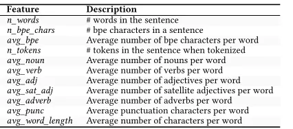
Table 7. All features considered for machine translation. See Section3.5
Feature Description
n_words # words in the sentence n_bpe_chars # bpe characters in a sentence
avg_bpe Average number of bpe characters per word n_tokens # tokens in the sentence when tokenized avg_noun Average number of nouns per word avg_verb Average number of verbs per word avg_adj Average number of adjectives per word avg_sat_adj Average number of satellite adjectives per word avg_adverb Average number of adverbs per word avg_punc Average punctuation characters per word avg_word_length Average number of characters per word
Table 8. Correlation values (absolute) of removed features to the kept ones for machine
translation.
Kept Feature Removed Feature Correl.
n_bpe_chars 0.96
n_words n_tokens 0.99
newstest dataset [60] to create ourpremodeltraining data. Using10-fold-cross-validationon our
premodelto give a end-to-end analysis of our approach.
6.1 Premodel for Machine Translation
6.1.1 Feature Selection.We considered a total of 11 features, which can be seen in Table7, and
a Bag of Words (BoW) representation of each sentence (explained in more detail below). Similar to
image classification, we chose our candidate features based on previous work [29,36],e.g.BoW, as
well as intuition based on our motivation (Section2.1),e.g. n_words(longer sentences are more
complex and require a more complex translator).
Bag of Words.Applying our method to machine translation brings with it the need to classify each
sentence to predict the optimalDNN. Text classification is a notoriously difficult task, and is made
more difficult when we only have a single sentence to gather features from. We are able to create a
successfulpremodelonly using the features described in Table7. However, with the addition of a
Bag of Words (BoW) representation of each sentence we saw an increase in accuracy. Furthermore,
previous work in sentence classification [29,36,38] often use a BoW representation, suggesting
that BoW can be useful for characterizing and modeling a sentence. A BoW representation of text describes the occurrence of words within the text. It is represented as a vector that is based on a vocabulary. We generated a domain specific vocabulary based on all words in our training dataset. Finally, we used Chi-square (Chi2) to perform feature reduction, which is widely used for BoW, leaving us with a BoW feature vector of length 1500. We include a full evaluation of the effect of
BoW and Chi2 feature selection on our machine translationpremodelin Section7.3.2.
Table8summarizes the features we removed during the first stage of feature selection, leaving
9 features. During the second stage we reduced our feature count down to 3 features (see Table6).
Figure9b summarizes the accuracy loss by removing any of the three selected features; the two
shown in Table6, and a BoW representation. It can be seen that by including BoW we reach a much
higher accuracy. This is to be expected, as BoW is a well researched and used representation of text
input. If we remove eithern_wordsoravg_adjthere is a small drop in accuracy, this indicates that
BoW is able to capture similar information. We chose to keep both of these features as they bring a small increase to accuracy with negligible overhead.
6.1.2 Creating The Premodel.Using our approach resulted in implementing a singleNBclassifier
premodel. We believe that a single architecturepremodelwas chosen because of our reduced
dataset,i.e.we have one tenth of the training data compared to image classification.NBachieved a
high accuracy for this task, and has a quick prediction time (<1ms).
Applying our Model Selection Algorithm, we setselection_methodto ‘Accuracy’ andθto 2.0.
Optimizing Deep Learning Inference on Embedded Systems Through Adaptive Model Selection:15
3 _l a y e r
g nm t_ 2 _ l ay e r
g nm t_ 8 _ l ay e r
O ur A p pr o a
c h O ra c l
e
0
5 0 0 1 0 0 0 1 5 0 0 2 0 0 0
In
fe
re
n
c
e
T
im
e
(
m
s
)
3 _l a y e r g nm t
_ 2_ l a y e r g nm t
_ 8_ l a y e r O ur A
p pr o a c h
O ra c l
e
0
2
4
6
J
o
u
le
s
3 _l a y e r g nm t_ 2
_ l ay e r g nm t_ 8
_ l ay e r O ur A
p pr o a c h
O ra c l
e
0
1 0 2 0 3 0 4 0 5 0 6 0
7 0 B L E U R o u g e F 1
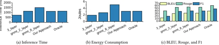
[image:15.486.55.421.87.163.2](a) Inference Time (b) Energy Consumption (c) BLEU, Rouge, and F1
Fig. 10. Machine Translation – Overall performance of our approach against individual models and anOracle.
selection ofgnmt_2_layer,gnmt_8_layer, andgnmt_3_layerforModel-1,Model-2, andModel-3,
respectively. Finally, we use the training data generated in Section6.1.1and 10-fold-cross-validation
to train and evaluate ourpremodel.
6.2 Overall Performance for Machine Translation
In this section, we evaluate our methodology when applied to Neural Machine Translation (NMT).
We compare our approach to 3 otherNMTmodels we considered in ourpremodel, we chose the
selected models as they show a range of complexity and capability. Furthermore, we compare our
approach to anOracle, atheoreticalperfect predictor that achieves the the best possible score for
each of out evaluation metrics.
6.2.1 Inference Time.As depicted in Figure10a,3_layeris the quickestDNN, 1.55x faster than the
Oracleand 2.05x faster than the most complex individualDNN,gnmt_8_layer. However,3_layer
is also the least accurateDNN(Figure10c) as it is outperformed in every accuracy metric by all
other approaches. Our approach, theOracle, andgnmt_2_layerhave very similar inference times;
nonetheless, our approach and theOracleoutperformgnmt_2_layerfor accuracy. The runtime
of ourpremodeland feature extraction is small, consisting of <1ms for thepremodeland <5ms for
feature extraction, per sentence. Feature extraction andpremodeloverheads are included in the
inference time of our approach and theOracle. Incidentally, our approach is slightly quicker than
theOracle; this is a result of ourpremodeloften mispredictinggnmt_2_layerforgnmt_8_layer
and vice versa. This specific misprediction makes up 38.5% of the cases wherepremodelmakes
an incorrect prediction. To improve accuracy we will need more data to train ourpremodel, as
we currently have a high feature to sentence ratio. Alternatively, we could deeply investigate the
sentences that are best for each model and intuitively add a new feature to ourpremodel, however,
the differences may not be intuitive to spot. Overall, we are 1.34x faster than the single most capable
DNNwithout a decrease in accuracy.
6.2.2 Energy Consumption.Figure10b compares energy consumption, includingpremodelcosts,
which are negligible (See Section7.4). Much like the image classificationDNNs, energy consumption
is proportional to model inference time; therefore, as we reduce overall inference time we also improve energy efficiency. A major difference between energy consumption and inference time is
the emphasised ratios between each model,e.g.gnmt_2_layeris 1.24x quicker thangnmt_8_layer,
but it uses 1.90x less energy, nearly half as much. Overall, we use 1.39x less energy on average than the single most capable model, without a significant change in F1 measure. Therefore, our methodology can be used to improve energy efficiency while having little impact on accuracy, or
in some cases, seeing an improvement in accuracy. Furthermore, ourpremodelis able to predict
when none of theDNNsare able to give a suitable output, in this case we can skip inference to avoid
wasting power. Implementing this results in using 1.48x less energy on average thangnmt_8_layer.
6.2.3 BLEU, Rouge, and F1 Measure.Figure10c comparesDNNsacross our accuracy metrics. We
CN
N
SV
M
De c is i
on T r ee
s
KN
N
dt . s vm
. dt k n
n. d t .d
t
s vm . dt .
dt dt . k nn
. dt
k nn . sv m
. dt
s vm . sv m
. dt
dt . s vm
. sv m dt .k n n. s
v m k nn
. dt . s vm dt .
k nn . kn
n
s vm . dt .
s vm
k nn . sv m
. sv m dt .s v m. k
nn
s vm . sv m
. sv m k nn . kn
n. d
t
dt . dt .
k nn s vm
. kn n. d
t
k nn . dt .
k nn dt . dt .d
t
k nn . sv m
. kn
n
s vm . dt .
k nn dt . dt .s v
m
s vm . sv m
. kn
n
k nn . kn
n. s v m
s vm . kn
n. s v m
s vm . kn
n. k nn
k nn . kn
n. k nn 0 . 0
0 . 1 0 . 2 0 . 3 0 . 4 0 . 5
0 . 6 T i m e T o p - 1 P e r c e n t a g e
T im e ( s ) 5 5 6 0 6 5 7 0 7 5 8 0 8 5 9 0 T o p -1 P e rc e n ta g e
F ea t u re
S ta c k in g
Mu l t i DT
S in g l e D
T
Mu l t i K N
N
S in g l e K
NN Mu lt i
S VM Mu l
t i NB S in g
l e S V M
S in g l e N
B
0
2 0 0 4 0 0 6 0 0 8 0 0 1 0 0 0 1 2 0 0
1 4 0 0 I n f e r e n c e F 1
In fe re n c e ( m s ) 3 5 3 6 3 7 3 8 3 9 4 0 F 1
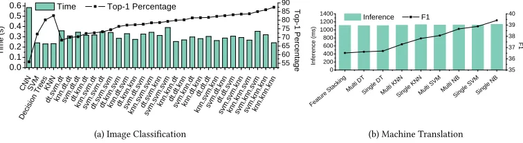
[image:16.486.54.432.86.190.2](a) Image Classification (b) Machine Translation
Fig. 11. Comparison of alternative predictive modeling techniques for building thepremodel.
not fail on the same sentences, we are able to achieve an overall better F1 measure by leveraging
multipleDNNs. This can be seen by looking at theOracle, which achieves an F1 measure of 47.54,
a 20% increase overgnmt_8_layer, which achieves 39.71. For this case study, we achieved 83% of
theOracleF1 measure. Overall our approach achieves approximately the same F1 measure as the
single most capable model, and improves upon the accuracy ofgnmt_2_layer(the closest single
DNNin terms of inference time), by 4%. For ourpremodelto achieve its full potential, as show by
theOracle, we require more data to train and test ourpremodel.
7 ANALYSIS
We now analyze the working mechanism of our approach to justify our design choices.
7.1 Alternative Techniques for Premodel
7.1.1 Image Classification.Figure11a shows the top-1 accuracy and runtime for using different
techniques to construct thepremodel. Here, the learning task is to predict which of the inference
models,MobileNet,Inception, andResNet, to use. In addition to our multi-classifier architecture
made up of onlyKNNclassifiers, we have considered different variations of Decision Trees (DT) and
Support Vector Machines (SVM). We also consider a single architecturepremodelusing the above
mentionedMLtechniques, and aCNN. OurCNN-basedpremodelis based on the MobileNet structure,
which is designed for embedded inference. We train all models using the same examples. We also
use the same feature set forKNN,DT, andSVM. For theCNN, we use an automated hyper-parameter
tuner [31] to optimize the training parameters, and we train the model for over 500 epochs.
Notation.In this instance, our multiple classifier architecture requires 3 components. We denote a
premodelconfiguration asX.Y.Z (see also Section3.2.1), whereX,Y andZindicate classifier for
the first, second and third level of thepremodel, respectively. For example,KNN.SVM.KNNdenotes
using aKNNmodel for the first and last levels, with aSVMmodel at the second level.
While we hypothesized aCNNmodel to be effective, the results are disappointing given its high
runtime overhead. AKNNmodel has an overhead that is comparable to theDTand theSVM, but has
a higher accuracy. It is clear that our chosenpremodelarchitecture (KNN.KNN.KNN) was the best
choice, it achieves the highest top-1 accuracy (87.4%) and the fastest running time (0.20 second).
One of the benefits of using aKNNmodel in all levels is that the neighbouring measurement only
needs to be performed once as the results can be shared among models in different levels;i.e.the
runtime overhead is nearly constant if we use theKNNacross all hierarchical levels. The accuracy
for each of ourKNNmodels in ourpremodelis 95.8%, 80.1%, 72.3%, respectively.
7.1.2 Machine Translation.Figure11b shows the F1 measure and inference time for different
architectures ofpremodelwhen applied to the machine translation problem. In this instance, we
Optimizing Deep Learning Inference on Embedded Systems Through Adaptive Model Selection:17
O pt i m a l -5 . 0
O pt i m a l -2 . 0
O pt i m a l -1 . 0
O pt i m a l -0 . 5 A l te r n
a t e- 5 .0 A l te r n
a t e- 2 .0 A l te r n
a t e- 1 .0 A l te r n
a t e- 0 .5 A cc u ra c y
- 5 .0 A cc u ra c y
- 2 .0 A cc u ra c y
- 1 .0 A cc u ra c y
- 0 .5
0
2 0 0 4 0 0 6 0 0 8 0 0
1 0 0 0 M e a n R u n t i m e T o p - 1 A c c u r a c y
M
e
a
n
R
u
n
ti
m
e
(
m
s
)
0
2 0 4 0 6 0 8 0 1 0 0 T
o
p
-1
A
c
c
u
ra
c
y
(
%
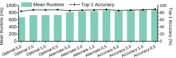
[image:17.486.155.333.83.142.2])
Fig. 12. The inference time and Top-1 accuracy achieved when building apremodelbased on the Model
Selection Algorithm configurations shown.
input sentence. Ourpremodelcan also predict that all these translators will fail, making a total
of 4 labels to choose from. We evaluated single and multiple architectures, acrossKNN,DT,SVM, and
NBclassifiers. For multiple classifier architectures we carried out a less exhaustive search compared
to Section7.1.1; we discovered that best performance was often achieved by using the same classifier
for each component. Finally, we compare an alternate approach named feature stacking [36]. Using
feature stacking we split classification into two classifiers, one using the BoW features, the other using our remaining features, we then use a probability measure choose the predicted model.
For this problem we can see that the single classifier architecture always outperforms its multiple classifier alternative. This is likely as a result of our high dimensional feature space, with a comparatively low training set. Feature stacking also had a poor performance for this problem, in fact it performs worse than all other architectures, indicating that our features work better together. Overall, there is little variance in the runtime of each approach, every model achieves a
runtime between 1100ms and 1140 ms. Our chosen approach, a singleNBclassifier, achieves the
highest F1 measure overall, with very similar runtime to all other approaches.
7.2 Sensitivity Analysis for Model Selection Algorithm
In Section3.3, we describe the algorithm we created to decide whichDNNsto include in ourpremodel.
In this section we will analyze how changing the parameters given to the Model Selection Algorithm
effect ourpremodel, and the resultant end-to-end performance. We will perform a case study using
image classification, but the results for machine translation are very similar. We consider the
performance if we were able to create a perfect predictor as apremodel, this is to prevent our
premodelaccuracy from introducing any noise and allowing us to evaluate the Model Selection
Algorithm in isolation. a total of 12 parameter configurations – our three available choices for SelectionMethod(defined in Section3.3), and 4 different choices forθ(5.0, 2.0, 1.0, and 0.5). We take every combination of these parameters.
Notation.Our parameter configuration is SelectionMethod-θ, whereSelectionMethod is either Accuracy, Optimal, orAlternate; andθ is our threshold parameter. For example, the notation Accuracy-5.0, means we always select the most accurate model in each iteration of our algorithm, and we stop once our accuracy improvement is less than 5.0%.
7.2.1 Results.Figure12shows the effect of different parameters on our finalpremodelresults. As
we decreaseθ, our Model Selection Algorithm will select more models to include in ourpremodel,
e.g.ThepremodelofAlternate-5.0to Alternate-0.5is made up of 3, 4, 5, and 7 DNNclassifiers,
respectively. Including moreDNNsresults in a higher overall top-1 accuracy, however there are also
some drawbacks. MoreDNNsmeans more classes for ourpremodelto choose between, therefore
making the job of thepremodelharder. It also means that we need to hold moreDNNsin memory,
which could be an issue for devices with limited memory (We discuss resource usage in more detail
in Section7.6.2). It is worth noting that there is no change inDNNselection fromOptimal-2.0to
Optimal-1.0, as the next model that we can add only brings an accuracy improvement of 0.488.
Finally, we can see that eachSelectionMethod has its own ’profile’, that is, each has its own
positive and negative impact. Figure12shows thatOptimalresults in an overall faster runtime,