Developing a Neuro Fuzzy Model for Weather Prediction

Developing a Neuro-Fuzzy Model for Weather Prediction

Hatem Mohamed Abd EL-Kader

Information Systems Department Faculty of Computers and Informatio, Manoufia

University, Egypt

Amr Ibrahim Awd El-Shora

Lecturer of Computer Science

Higher Institute of Management and Information Technology, Kafrelsheikh, Egypt

ABSTRACT

The vast weather changes effect on human activities. Dealing with weather data manually is very difficult job and time consuming operation. The process of data entry requires a precise method suits different weather parameters. Artificial intelligent [AI] especially, hybrid systems improve the performance of either pure neural network based or pure fuzzy logic based forecasting. In this study, a Neuro-fuzzy approach will be proposed to predict weather in Sadat region, western desert, Egypt. A combination of monthly mean meteorology measurements for temperature, relative humidity, wind speed, and rainfall will be used during the period [2008-2017]. Many methods were applied over the years for weather prediction such as classical and intelligent techniques. The proposed model uses a Neuro-fuzzy model at different types of fuzzy member ship functions. The flexibility of the proposed model increase the prediction accuracy. The effectiveness of the proposed model is demonstrated at different operating conditions. The classification of data is divided into 12 sets; each set consists of 4 mean values of observations. A transposing process applied on these sets for training and testing at different number of rules 10, 11, 15, 20, 25, 30, 35, and 40. Eight choices for membership functions "triangular" and another for "Gaussian" performed. The accuracy of the output forecasting measured using MAPE and MAE. A comparison applied among different cases obtained from Neuro-fuzzy model and observed meteorological data for year 2017. The results show that the performance of the Neuro-fuzzy model at TCWB is better than TLWB. Also, the model at GCWB and GCWN are better than GCCB and GCCN. The results show that Neuro-fuzzy model seemed to be promising method for weather prediction.

Keywords

Weather predication, Neuro-fuzzy,

1.

INTRODUCTION

Weather prediction is an application of technology and computer science to predict the state of weather for a future time in a certain location. People have attempted to predict the weather informally since long time,. Weather prediction are made by gathering quantitative data about the current state of the atmosphere and using scientific understanding of weather evolving processes to indicate how the atmosphere will evolve. Manual input is still required to get the best possible predication model to base the expectation upon, which involves pattern recognition tasks, knowledge of model performance, and accuracy.

There are a variety of end users to weather predication . Weather warnings are important forecasts because they are used to protect life and property. Forecasts based on temperature and pressure are important to agriculture, and therefore to traders within commodity markets. Temperature forecasts are used by utility companies to estimate demand over coming days. People use weather predication to

determine what to dress on a given day. Since outdoor activities are strongly reduced by heavy rain, snow and the wind. Also weather predication can be used to organize activities around these events, and to plan ahead and survive them.

Fundamentally, there are only two methods to predict weather: the empirical approach and the dynamical approach [18]. The empirical approach is based upon the occurrence of analogs and referred to meteorologists as analog forecasting. This approach is useful for predicting local-scale weather if the recorded cases is plentiful.

The dynamical approach is based upon equations and forward simulations of the atmosphere and referred to as computer modeling. This approach is only useful for modeling large-scale weather phenomena. In practice, most weather prediction systems used a combination of empirical and dynamical techniques.

Weather prediction presents severe challenges for AI. Weather is continuous; data are intensive, multidimensional, dynamic and chaotic. For these properties, weather prediction was proving ground for any AI prediction system. The operational weather forecasting involves the application of accumulated human expertise. There are three aspects of forecasting that should be considered when developing intelligent systems for operational meteorologists. First, forecasting relies on a variety of techniques. Second, experts convey their knowledge with fuzzy terms. Third, data are often imprecise [14].Artificial intelligent systems require some modifications to be price adopted operation. Modeling weather date have to performed via two steps the first is optimization process to choose the best and low cost models that have the capabilities to deal with a large number of climate parameters. The second step is, modeling of actual environmental data related to various environmental applications which needs detailed studies for investigating the suitable model for each application

In [30], It was declared that Fuzzy Logic lets people compute with words. He stated that there are two major imperatives for computing with words. First, if the available information is too imprecise to justify the use of numbers. Second, when there is flexibility for imprecision which can be used to achieve tractability, robustness, low solution cost, and better rapport with reality?

It was stated in [14] that there is no single AI technique favorable for all meteorological applications. When AI methods are hybridized in a system, the system can inherit the strengths of its constituent AI methods.[11] applied a linear filter model, moving average model, to thirty years of Alexandria rainfall. They showed that there may be severe rainfall in some years, moderate rainfall at some years, drought and light rainfall at the other years.[9] applied a model to predict yearly, seasonally and some squalls sum of rainfall in Arish and Helwan during the period 1968 to1997. They concluded that there may be big amount of rainfall in years 2000, 2005 and a moderate rainfall in year 2002. This study aimed to propose an information system based Neuro-fuzzy model to deal efficiently with large sized weather observations in order to predict the weather changes in Sadat region, western desert, Egypt.

The paper is organized into six sections. The first section gives an introduction. Section two covers the related works. Section three will be introduce the proposed model. The methodology of proposed model implementation is given in section four. Simulation results are given in section five.

Finally the conclusions are drawn in section six.

2.

RELATED WORKS

Several methods were applied over the years for weather prediction such as classical and intelligent techniques [Fig.1]. Many other hybrid systems proposed such as Neuro-Expert [KB-NN], Neuro-Genetic [NG], Neuro-Fuzzy [NF] and Fuzzy-Genetic [FG] methods. Pure FL systems suffer from the lack of a specific method to determine membership functions, and the lack of learning capability that can be overcome by NNs driven by fuzzy reasoning. To improve the performance of either pure NN-based or pure FL-based forecasting, several combinations of NN and FL systems were applied. Neural networks are used in NF systems to tune the membership functions of the fuzzy variables involved. On other words, to adjust the fuzzy sets [linguistic labels] and determine the membership functions. FL can convert expert knowledge directly into fuzzy rules, but it takes a lot of time to design and adjust the fuzzy sets. NF systems possess improved performance and reduced trial-and-error waste time. This is achieved via the learning of the NN [27].

Fig.1: The diagram of different prediction techniques.

There are three classical Neuro-Fuzzy systems. First is Adaptive Neuro-Fuzzy Inference System [ANFIS]. Second is Generalized Approximate Reasoning-based Intelligent Control [GARIC]. Third is Fuzzy Adaptive Resonance Theory [Fuzzy ART] system.

It was shown in [6] that neuro-fuzzy systems are a powerful trade off in terms of reliability and efficiency between a human-like representation of the model and a fast learning method. However, what mainly differentiates Neuro-fuzzy estimators from other kinds of non linear approximates is their potentiality for combining available a priori first principle models with data driven modeling techniques. In fact, while learning methods provide the adaptation of the inference system to the observed data, the fuzzy architecture allows an easy integration into the system of available knowledge about the process to be modeled.

Also in it was shown in [12] that neural networks can be used for long range forecast for rainfall in region called Matroh, Egypt. They deduced that the data predicted from applying the back propagation algorithm are more accurate than the data predicted from applying the statistical model. In [24] the authors concluded that querying a large database of weather observations for past weather cases similar to a present case

using a fuzzy similarity measure can increase the accuracy of predictions of cloud ceiling and visibility at an airport. It was shown in [17] that the applicability of an ensemble of neural networks and learning paradigms for weather forecasting in Canada. They proposed ensemble method for weather forecasting which has advantages over other techniques like linear combination. The data of temperature, wind speed and relative humidity are used to train and test the different models.

It was shown in [23] that a framework for a statistical anomaly prediction system using a neuro-genetic forecasting model.

It was shown in [3] that the predictability of a recent version of the European Center for Medium-Range Weather Forecasting [ECMWF] model. They used two different estimates of the initial error corresponding to 6- and 24-hr forecast errors, respectively. [26] concluded that the annual or seasonal variability had a high spatially and temporary variance. He stated that it is recommended to give attention for the long range forecasting of rainfall over Egypt.

It was shown in [29-31] that the meteorological characteristics of Mount Everest during the observational 10-minute mean and daily records temperature, minimum temperature, maximum temperature, relative humidity, pressure and wind speed.

It was shown in [1] that the Doppler radar data assimilation improves the initial field and enhances the Quantitative Precipitation Forecasting [QPF] skill.

It was shown in [16] that a model to study a heavy rainfall event along the west coast of India. The model is a next-generation musicale numerical weather prediction system designed to serve both operational forecasting and atmospheric research communities.

Nearest Neighbor Based Fuzzy Model [NNFM] based on membership values was used in [21] to forecast the daily maximum temperature at Delhi. He found that this method is promising for operational application. [2] built an effective grid-based problem solving environment that truly extends and embraces a computational scientist’s traditional tools are multifold. They have focused on the most challenging users of numerical weather prediction.

A method of classification of weather forecasts in was proposed in [20] , this is done by applying fuzzy grade statistics. Also , it was reported in [21] , that the advantages of artificial neural network technique for explaining the nonlinear behavior between the inputs and output is explored to forecast the monsoon rainfall of 36 meteorological sub-divisions of India

It was proposed in [22] that a spatially explicit seasonal forecasting based on the fuzzy classification of long-term [40 years] daily rainfall and temperature data to create climate relations over time and location.

It was stated in [7] that over the last few years, global weather forecasts from a number of operational numerical weather prediction centers continued to progress steadily in skill and reach an impressive level of quality.

3.

THE PROPOSED MODEL

3.1. Study Area:

Sadat region has a unique location between Cairo and Alexandria and adjacent Delta making it a center for attracting domestic and foreign investments. It lies west of the Nile Delta and eastern side of the Cairo-Alexandria desert road from kilo 85 to 109. It is bounded by longitude 30° 21' 64" - 30° 39' 55" E and latitude 30° 18' 57" - 30° 38' 19" N. It divided into four major zones including housing zone, industrial zone, cultivated and non-reclaimed zone. It characterized by a long hot summer and a short warm winter, low rainfall rates 15-25 mm/ year [see Figure .2].

3.2.Data Used:

The data used is a database of weather observations consist of temperature [T], relative humidity [H], wind speed [W] km/h, and rainfall [R] mm. These parameters are meteorological data of daily weather observations during the period from

2007 to 2016. The rainfall data is a monthly mean weather observation during the same period.

3.3. Software Package:

The technique used is a neuro-fuzzy which integrated a model structure based on fuzzy production rules and a tuning procedure inspired by neural networks. The toolbox used is a neuro-fuzzy identification and data analysis. It was tested in Matlab . It performs the identification of a Takagi-Sugeno [TS]fuzzy architecture starting from a set of N input-output samples [5]. The TS fuzzy model was proposed to develop a systematic approach to generating fuzzy rules from a given input-output data set.

3.4. From Fuzzy to Neuro-Fuzzy:

A TS fuzzy inference system is a set of r rules:

If x1 is 1 1

A

_{and x2 is}

A

1_{2 … and xn is}

A

1n _{then y= f[x1,}

x2,…, xn]………. [1] ……… ………

If x1 is

r

A

₁

and x2 is

r

A

_{2…and xn is}

A

nr _then r

y

=

r

f

[x1, x2,…, xn]………. [2]

The first part [antecedent] of each rule is defined as a fuzzy AND proposition where

i j A

is a fuzzy set on the jth premise variable defined by the membership function





0,1

:Rn  i

j



. The second part [consequent] is a crisp function

i

f

;i=1, …, r of the input vector [x1, x2, …, xn]. By

means of the fuzzy sets

i j

A

the input domain of the function f is softly partitioned in smaller regions where the mapping is locally approximated by the models

i

f

.

The TS inference system uses the weighted mean criterion to recombine all the local representations in a global approximator:









_i

r

i i i

y

y





1

[3]

where



i is the degree of fulfillment of the ith rule.

In a conventional fuzzy approach the membership functions and the consequent models are fixed by the model designer according to a priori knowledge. If this knowledge is not available but a set of input-output data is observed from the process f , the components of the fuzzy system [membership and consequent models] can be represented in a parametric form and the parameters tuned by a learning procedure. In this case, the fuzzy system turns into a neuro-fuzzy approximator [6].

3.5.Structural and parametric learning in

NF systems:

satisfactory structure, the parametric tuning searches for the optimal membership functions together with the optimal parameters of the consequent models. The number of rules selected as a measure of complexity to be properly tuned on the basis of available data. An incremental approach was adopt where different architectures having different number of rules. This approach assessed in cross-validation and then compared in order to select the best one. The whole learning procedure is represented in the flow chart [Fig.3].

The initialization of the architecture is provided by a hyper-ellipsoidal fuzzy clustering procedure. This procedure clusters the data in input–output domain obtaining a set of hyper-ellipsoids which are a preliminary rough representation of the input-output mapping. This procedure used the axes of the ellipsoids to initialize the parameters of the consequent functions f i.The cluster centers were projected on the input domain to initialize the centers of the antecedents. The scatter matrix adopts to compute the width of the membership functions. An example of fuzzy clustering in the case of a single-input/single-output function modeled by a fuzzy inference system with Gaussian antecedents [Fig.4]. Once the initialization is done, the learning procedure begins. Two optimization loops are nested: the parametric and the structural one. The parametric loop [the inner one] searches for the best set of parameters by minimizing a sum-of-squares

cost function JM which depends exclusively on the training

set. The structural identification loop [the outer one] searches for the best structure, in terms of optimal number of rules, by increasing gradually the number of local models.

The toolbox has a graphical interface [Fig. 5]. It is called by typing command fuzzy_g at command window. The program provides a set of structural alternatives in the definition of the fuzzy model. The user may choose Shape of the membership functions of the antecedents: it can be gaussian or triangular. Parametric form of the consequent model: it can be constant or linear. Combination method of the rules: it can be a weighted combination or a non weighted combination. Bias term: it can be used or not in the linear step of the nonlinear parametric optimization. Clustering initialization policy: it can be k_mean or Hyperplane Fuzzy Clustering [HFC].

3.6. Training, Model Selection and

Prediction:

The training set is a .mat file containing a rectangular matrix [N, n+1] named data. The number N represents the number of training samples. The value n is the number of inputs and the last column of the matrix data contains the training output. The number of output is always restricted to one. This matrix must be saving in a file .mat

Fig.4: The hyper-ellipsoidal clustering initialization procedure [6].

The input samples for which a prediction required must be formatted in a matrix [Nts, n] named in. The number Nts is the

number of samples for which a prediction is required while n

is the number of inputs which has to be the same as the number used in the training set. This matrix must be saving in a file .mat.

Fig.5: The graphical interface of neuro-fuzzy model [5].

4.

METHODOLOGY

4.1. Stage of preparing the data:

This stage carried out during the following steps:

1- Calculate the arithmetic mean for every month for every year [2009-2016] of weather observations temperature, relative humidity, wind speed and rainfall.

2- Compute the standard deviation for previous data. 3- Calculate the sum of pollen grains for every month

during the year. Divide its value for every month by this sum to obtain the percentage of month with respect to year.

4- Obtain the maximum and minimum values of weather observations and pollen grains for every year. 5- Calculate the arithmetic mean for the four seasons

[winter through autumn] during ten year [1999-2008] of weather observations.

6- Classify the data into 12 sets, each set consist of four means observations [T,H,W,R] for one month of 12 months and this are applied for 10 years.

7- Transpose these sets into 10 columns each column contains 48 values represent one year. The first 9

columns for period [1999-2007] for training. The 10th column will be used to compare the actual and the forecasted values of year 2008.

4.2. Stage of Training and Model Selection:

From the previous section, the number of training samples N equal to 48. Also, the number of inputs n equal to 9. The last column of the matrix data contains the training output. Starting with Matlab® [Version 7.0], then at command window we type the following commands:

N=48; inputs=[48,9]; output=[48,1]; data=[inputs output]; Save data_example data;

The matrix saved in a file, namely data_example.mat. At command window, type the command fuzzy_g. The neuro-fuzzy toolbox appeared. Apply and change the fixed parameters of the model [independent variables] as follow:

1- Choose the option “Train one model of a given complexity”.

2- Click on button “Get data from”to read data file data_example.mat

3- Choose number of rules [notice that it settled to 9]. 4- Set the shape of the membership functions of the

5- Set the parametric form of the consequent model to“Linear”.

6- Choose the combination method of the rules“Weighted”.

7- Bias term [used].

8- Choose the Clustering initialization policy “HFC”. 9- Click ok.

The trained model has been saved in the file model.matand diary of the computation has been saved in the filemhist.txt.The file namely, model.mat includes the created model which will use for the process of prediction.

4.3. Stage of Prediction:

From the previous section, the input samples for which a prediction required was a matrix [48, 9] named in. Starting with Matlab® [Version 7.0], then at command window we type the following commands:

N=48; in=inputs; Save test_example in;

The matrix saved in a file, namely test_example.mat. At command window type the command fuzzy_g. The neuro-fuzzy toolbox appeared and then, applies the following steps:

1- Choose the option “Evaluate an existing model”. 2- Choose “Get model from” to provide the program with

the model trained in the previous section, namely model.mat.

3- Set the input samples by choosing “Get Inputs from” to read data file namely, test_example.mat.

4- Click ok.

[image:6.595.90.511.311.614.2]

The predicted output has been saved in the fileout_hat.matand the program will return the set of predictions in the default file namely, out_hat.mat. This file is about excel sheet has the same length 1 column and 48 rows. The same steps repeated after change the setting and using different number of rules [10, 11, 15, 20, 25, 30, 35, and 40]. Eight options applied for membership functions “triangular” and others for “Gaussian” [table 1].

Table [1]: The different options of neuro-fuzzy model.

No. Membership functions Parametric form of consequent model

Combination

method of rules Bias term

1

Triangular

Linear

Weighted

Bais

2 No Bais

3

Combined

Bais

4 No Bais

5

Constant

Weighted Bais

6 No Bais

7

Combined

Bais

8 No Bais

9

Gaussian

Linear

Weighted

Bais

10 No Bais

11

Combined Bais

12 No Bais

13

Constant

Weighted

Bais

14 No Bais

15

Combined

Bais

16 No Bais

4.4. Stage of Prediction Accuracy:

Several criteria were used to measure the quality or accuracy of the forecasting. The following error criterion applied in this study:

4.4.1. Mean Absolute Error [MAE]:

MAE =







N

i

i

forecat

i

actual

N

1

)

(

)

(

1

, where N is the total number of data points, actual [i] is the ith

actual value, and forecast[i] is the ith forecast.

4.4.2. Mean Absolute Percentage Error [MAPE]:

MAPE =

%

100

)

(

)

(

)

(

1

1









N

i

actual

i

i

forecat

i

actual

N

, where N is

the total number of data points, actual [i] is the 1th actual value, and forecast [i] is the ith forecast.

5.

RESULTS

5.1. Parameters Before Importing To

Model:

Table 2 and Fig.6 show that the mean of temperature was lowest value at January and equal to 12.31 C ْ with standard

division [sd] equal to 0.88. Also, it was highest value at August and equal to 26.2 C ْ with sd equal to 0.42.

The mean of relative humidity was lowest value at April and equal to 65.28 % with sd equal to 3.31. Also, it was highest value at January and equal to 74.02 % with sd equal to 6.07 [Table 2; Figure.7].

Fig.6: The monthly mean of temperature during years 1999-2008

Fig.7: The monthly mean of relative humidity during years 1999-2008

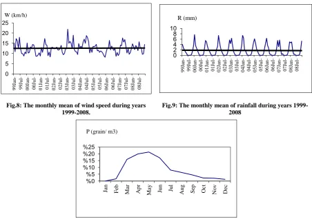
The mean of wind speed recorded lowest value at October and equal to 9.41 km/h with sd equal to 0.81. Also, it was highest value at April and equal to 14.95 km/h with sd equal to 1.59 [Table 2; Fig.8].

Table 2 and Fig.9 show that the mean of rainfall was lowest value at October and equal to 0.5 mm with sd equal to 0.18. Also, it recorded highest value at January and equal to 5.62

mm with sd equal to 1.58. No rainfall data recorded during June through September.

Table 3and Figure.10 show that the percentage of pollen grains was lowest value at February and equal to %. Also, it recorded highest value at May and equal to 21.29%. There are no values for it at January.

Fig.8: The monthly mean of wind speed during years 1999-2008.

Fig.9: The monthly mean of rainfall during years 1999-2008

Fig.10: The monthly percentage of pollen grains during years 2006-2008

0 5 10 15 20 25 30 Ja n

-99 Jul

-99 Ja

n

-00 Jul

-00 Ja

n

-01 Jul

-01 Ja

n

-02 Jul

-02 Ja

n

-03 Jul

-03 Ja

n

-04 Jul

-04 Ja

n

-05 Jul

-05 Ja

n

-06 Jul

-06 Ja

n

-07 Jul

-07 Ja

n

-08 Jul

-08

T(Cْ )

0 10 20 30 40 50 60 70 80 90 Jan

-99 Ju

l-99 Jan

-00 Ju

l-00 Jan

-01 Ju

l-01 Jan

-02 Ju

l-02 Jan

-03 Ju

l-03 Jan

-04 Ju

l-04 Jan

-05 Ju

l-05 Jan

-06 Ju

l-06 Jan

-07 Ju

l-07 Jan

-08 Ju

l-08

RH(%)

0 5 10 15 20 25 Ja n -99 Jul

-99 Ja

n

-00

Jul

-00 Ja

n

-01

Jul

-01 Ja

n

-02

Jul

-02 Ja

n

-03

Jul

-03 Ja

n

-04

Jul

-04 Ja

n

-05

Jul

-05 Ja

n

-06

Jul

-06 Ja

n

-07

Jul

-07 Ja

n -08 Jul -08 W (km/h) 0 2 4 6 8 10 Jan -99 Jul

-99 Jan

-00

Jul

-00 Jan

-01

Jul

-01 Jan

-02

Jul

-02 Jan

-03

Jul

-03 Jan

-04

Jul

-04 Jan

-05

Jul

-05 Jan

-06

Jul

-06 Jan

-07

Jul

-07 Jan

-08 Jul -08 R (mm) 0 % 5 % 10 % 15 % 20 % 25 % Ja n

Feb Ma

r A p r Ma y Ju n Ju l A u g

Sep Oc

t N o v D ec

[image:7.595.162.510.147.317.2] [image:7.595.71.524.430.748.2]

Table [2]: The standard deviation of temperature, relative humidity, wind speed, and rainfall during ten years 1999-2008.

Months

Parameters

J

a

n

u

a

ry

Februa

ry

Ma

rc

h

April Ma

y

J

u

n

e

J

u

ly

Aug

u

st

S

ep

te

m

b

er

O

cto

b

er

No

v

em

b

er

De

ce

m

b

er

T [ C ْ] 0.88 0.74 1.2 0.47 0.56 0.77 0.63 0.42 0.78 0.59 0.73 0.44 H [ % ] 6.07 3.99 5.04 3.31 3.27 2.62 2.87 2.55 2.88 2.87 3.69 2.93 W [ km/h ] 2.21 3.19 2.02 1.59 2.24 2.23 2.79 2.49 1.95 0.81 1.3 2.26 R [mm] 1.58 1.3 0.53 0.57 0.12 0 0 0 0 0.18 0.5 0.96

Table [3]: The monthly mean and percentage of pollen grains during three years 2006-2008

Months

Mean &

Percentage

J

a

n

u

a

ry

Februa

ry

Ma

rc

h

April Ma

y

J

u

n

e

J

u

ly

Aug

u

st

S

ep

te

m

b

er

O

cto

b

er

No

v

em

b

er

De

ce

m

b

er

2006-2008 0 17 167.5 210 225 180 85 66.5 47.5 23.5 21.5 13.5 Percentage 0 1.61 15.85 19.87 21.29 17.03 8.04 6.29 4.49 2.22 2.03 1.28

5.2. Parameters after importing to model:

5.2.1. The model TLWB:

The predicted mean of temperature was a high accuracy [MAPE= 5.35%, 7.38%] at using number of rules [10, 25]. Also, itrecordedlowaccuracy [MAPE= 42.86%] at using number of rules [35]. So, this model is effective for temperature at number of rules [10, 25].

Also, at using number of rules [9, 25], the predicted mean of relative humidity was a high accuracy [MAPE= 4.44%, 4.61%].Also, lowaccuracy [MAPE= 45.28%]recorded at

using number of rules [40]. These results indicate that this model is effective for relative humidity at number of rules [9, 25].

The model was not suitable for wind speed where it gave low accuracy at all used rules. On the other hand, the predicted mean of rainfall was high accuracy [MAE= 6.68, 7.08] at using number of rules [35, 30]. Also, it recorded lowaccuracy recorded [MAE= 16.14] at number of rules [40] and no any prediction accuracy at the rest rules. This model is more effective for rainfall at two different values of rules [30, 35].

[a] [b]

TLWB

0% 20% 40% 60% 80% 100%

9 10 11 15 20 25 30 35 40

No. of rules

M

A

P

E T

RH W

0 % 10 % 20 % 30 % 40 % 50 % 60 % 70 % 80 % 90 % 100 %

9 10 11 15 20 25 30 35 40

M

A

P

E

No. of rules TLWN

[image:8.595.83.516.86.242.2] [image:8.595.72.531.517.705.2]

[c] [d]

Fig.11: MAPE of T, H & W at different number of rules using models[TLWB, TLWN, TLCB and TLCN]

5.2.2. The model TCWB:

In case of using number of rules [30, 9], the predicted mean of temperature was highaccuracy [MAPE= 0.86%, 4.26%] while it recorded low accuracy [MAPE= 52.38%] at using number of rules[35]. So, this model is effective for temperature at number of rules [9, 30].

Also, the predicted mean of relative humidity obtained at using number of rules [11, 10]was high accuracy [MAPE= 1.8%, 4.7%]. Also, it recorded lowaccuracy [MAPE= 38.9%] at using number of rules [40]. These results indicate that this model is more effective for relative humidity at using number of rules [10, 11].

In case of using number of rules [30], the predicted mean of wind speed was high accuracy [MAPE= 3.1%]. On the other hand, it recorded low accuracy [MAPE= 63.5%] at using number of rules [40]. These results showed that the model is more effective for wind speed at two different values of rules [30].

The predicted mean of rainfall was highaccuracy [MAE= 0.38, 0.44] at using number of rules [10, 11]. Also, lowaccuracy was recorded [MAE= 11.41] at using number of rules[40]. These results indicate that this model is more effective for rainfall at using number of rules [10, 11].

[a] [b]

[c] [d]

Fig.12: MAPE of T, H & W at different number of rules using models[TCWB, TCWN, TCCB and TCCN]

TLCB

0% 20% 40% 60% 80% 100%

9 10 11 15 20 25 30 35 40

No. of rules

M

A

P

E T

RH W

TLCN

0% 20% 40% 60% 80% 100%

9 10 11 15 20 25 30 35 40

No. of rules

M

A

P

E T

RH W

TCWB

0% 20% 40% 60% 80% 100%

9 10 11 15 20 25 30 35 40

No. of rules

M

A

P

E T

RH W

0 % 10 % 20 % 30 % 40 % 50 % 60 % 70 % 80 % 90 % 100 %

9 10 11 15 20 25 30 35 40

M

A

P

E

No. of rules TCWN

T RH W

TCCB

0% 20% 40% 60% 80% 100%

9 10 11 15 20 25 30 35 40

No. of rules

M

A

P

E T

RH W

TCCN

0% 20% 40% 60% 80% 100%

9 10 11 15 20 25 30 35 40

No. of rules

M

A

P

E T

5.2.3. The models GLWB, GLWN, GLCB, and

GLCN:

The MAPE results from using these models at all rules equal to zero and no change in values of used parameters before and after prediction. This may be due to some conflicts in used rules. Also, this may be due to use membership function “Gaussian”, consequent model “linear”, combination method of the rules “weighted or not” and bias term “used or not”which made these settings functionless.

5.2.4. The model GCWB:

The temperature prediction was achieved with highest accuracy [MAPE= 2.35%, 2.41%] at two different values of rules [35, 20] respectively, while the rest of results are accepted. So, this model is effective for prediction of temperature at all values of rules.

Also, the relative humidity prediction was obtained with high accuracy [MAPE= 0.32%, 0.67%] at two different values of rules [20, 15] respectively, while the rest results are accepted. So, this model is effective for prediction of relative humidity

at all values of rules.

A high accuracy for wind speed prediction [MAPE= 1.21%, 7.4%] was obtained at two different values of rules [35, 25] respectively, while the lowest accuracy [MAPE= 11.51%] was at values of rules 11. These results showed that this model is more effective for wind speed at two different values of rules [35, 25] and not effective at a value of rules equals 11.

For the rainfall prediction with highest accuracy [MAE= 0.07%, 0.28%] at two different values of rules [35, 10] respectively, while the rest results are accepted. These results indicated that the model is more effective for rainfall at all values of rules.

5.2.5. The model GCWN:

The model of the GCWN is effective for prediction of temperature; relative humidity, wind speed, and rain fall because it gives results slightly similar in accuracy to GCWB model.

[a] [b]

[c] [d]

Fig.13: MAPE of T, H & W at different number of rules using models[GCWB, GCWN, GCCB and GCCN]

5.2.6. The model GCCB:

The model is more effective for prediction of temperature at all values of rules except at two different values [15, 25] respectively where it gives lowest accuracy [MAPE= 12.73%, 11.56%].

Also, for the relative humidity prediction, it was found that the model is more effective for prediction at all values of rules

except at the following two values [15, 20] respectively, where it gives lowest accuracy [MAPE= 11.84%, 12.29%]. It was found that the model is more effective for all values of rules for wind speed except at the value [20] where it gave lowest accuracy [MAPE= 32.53%].

A lowest accuracy was obtained [MAE= 5.81%, 5.13%] at two different values of rules [15, 20] respectively for the

GCWB

0% 20% 40% 60% 80% 100%

9 10 11 15 20 25 30 35 40

No. of rules

M

A

P

E T

RH W

GCWN

0% 20% 40% 60% 80% 100%

9 10 11 15 20 25 30 35 40

No. of rules

M

A

P

E T

RH W

0 % 10 % 20 % 30 % 40 % 50 % 60 % 70 % 80 % 90 % 100 %

9 10 11 15 20 25 30 35 40

M

A

P

E

No. of rules GCCB

T RH W

0 % 10 % 20 % 30 % 40 % 50 % 60 % 70 % 80 % 90 % 100 %

9 10 11 15 20 25 30 35 40

M

A

P

E

No. of rules GCCN

rainfall prediction, while the rest results are more accepted.

5.2.7. The model GCCN:

The model gave the lowest accuracy [MAPE= 19.66%] at a value of rules [15] while it is more effective for prediction of temperature at the rest values of rules.

It was found that the model gave lowest accuracy [MAPE= 17.5%, 16.75%] at two different values of rules [11, 15] respectively for relative humidity prediction, while it is more effective at the rest number of rules.

For wind speed prediction, the model gave high accuracy levels [MAPE= 0.01%, 1.7%] at two different values of rules [35, 9] respectively, while the lowest accuracy [MAPE= 31.78%, 28.19%] at two different values of rules [15, 20]. These results showed that this model is more effective for wind speed at two different values of rules [35, 9] and it is not effective at two different values of rules [15, 20].

The highest accuracy for rainfall prediction was [MAE= 0.38] at value of rules [10], while the rest results were more accepted.

[a] [b]

[c] [d]

Fig.14: MAP of R at different number of rules using models [Triangular and Gaussian]

6.

CONCLUSIONS

By comparing the different cases of results from neuro-fuzzy model with the observed meteorological data and the accuracy of forecasting, it is found that the performance of the neuro-fuzzy model at TCWB is better than TLWB when the shape of membership function of the antecedents is triangular. Also, the models GCWB and GCWN are better than the models GCCB and GCCN when the shape of membership function of the antecedents is Gaussian.

The prediction of meteorological parameters such as temperature, relative humidity, wind speed, and rainfall using hybrid systems such as neuro-fuzzy model seemed to be promising method with successful test results.

Testing the models of prediction for climate changes is essential to verify the prediction process. It is logic to find climatically sensitive biological indicators such as pollen dust grains. Pollen dust was used in the current study to support the hypotheses of relativity of the pollen dust and the data of the climatic parameters. It was clear from the results that there is reverse relationship between pollen dust and rainfall, on other

words any rise in rainfall rates leads to decrease on atmospheric free pollen dust.

Also, there is relationship between pollen dust and wind speed, temperature, i.e. in case of increasing the wind speed and temperature this may leads to an increase on atmospheric free pollen dust. So, during winter season, where rainfall is recorded high we found low pollen dust counts were recorded. While during spring and summer seasons, where temperature is high and rainfall is low, it could be conclude that this may leads to rich atmospheric free pollen dust. This record supports the models of prediction in the current study.

7.

REFERENCES

[1] Abhilash, S., Das, S., Kalsi, S., Gupta, M., Mohankumar, K., George, J., Banerjee, S., Thampi, S., and Pradhan, D., 2007. Assimilation of Doppler weather radar observations in a mesoscale model for the prediction of rainfall associated with mesoscale convective systems, Journal of Earth System Science, V.116: 275-304.

[2] Alameda, J., Rossi, A.L., and Hampton, S., 2007. On the

0 2 4 6 8 10 12 14 16 18

9 10 11 15 20 25 30 35 40

M

A

E

No. of rules Rainfall

TLWB TLWN TLCB TLCN

0 5 10 15 20

9 10 11 15 20 25 30 35 40

M

A

E

No. of rules Rainfall

TCWB TCWN TCCB TCCN

Rainfall

0 2 4 6 8 10 12

9 10 11 15 20 25 30 35 40

No. of rules

M

A

E

GLWB GLWN GLCB GLCN

Rainfall

0 5 10 15 20

9 10 11 15 20 25 30 35 40

No. of rules

M

A

E

GCWB

GCWN

GCCB

use of services to support numerical weather prediction, International Federation for Information Processing. In: P.W. Gaffney and Pool, J.C.T., [Eds.], Grid-Based Problem Solving Environments, Boston: Springer, V.239: 339-348. [3] Bengtsson, L., and Hodges, K.I., 2006. A note on

atmospheric predictability, Tellus A, Blackwell Publishing, V.58: 154-157

[4] Bersini, H., and Bontempi, G., 1997. Now comes the time to defuzzify neuro-fuzzy models, Fuzzy Sets and Systems, Elsevier, V.90: 161-169.

[5] Bontempi, G., and Birattari, M., 1999. Toolbox for Neuro-Fuzzy Identification and Data Analysis For use with Matlab, Technical Report TR/IRIDIA/1999-009, IRIDIA, Université Libre de Bruxelles, Brussels, Belgium, 18p. [6] Bontempi, G., Bersini, H., and Birattari, M., 2001. The

local paradigm for modeling and control: From Neuro-Fuzzy to Lazy Learning, Neuro-Fuzzy Sets and Systems, Elsevier, V.121: 59-72.

[7] Bougeault, P., 2008. High performance computing and the progress of weather and climate forecasting. In: J.M.L.M. Palma et al. [Eds.], VECPAR 2008, LNCS 5336, Springer, pp. 349.

[8] Edwards, P.N., 2007. Atmospheric General Circulation Modeling.

[9] Eissa, M.M., and Hamada, E.M., 2001. Statistical models for long range forecast of Helwan rainfall, Meteorological Research Bulletin, Egyptian Meteorological Authority, V.16: 30-35.

[10]Eissa, M.M., and Salem, T.Z., 2000. Statistical models for long range forecast of Alexandria rainfall, The 5th conference on Meteorology and Sustainable Development, 22-24 February 2000, Egyptian Meteorological Authority, V.1: 282-292.

[11]Eissa, M.M., and Salem, T.Z., 2001. Statistical models for long-range forecast of Matrouh rainfall, Meteorological Research Bulletin, Egyptian Meteorological Authority, V.16: 36-41.

[12]El-Dahshan, K., Eissa, M.M., and Farag, M.S., 2001. Use of artificial neural networks based model for long range forecast of flashfloods, Meteorological Research Bulletin, Egyptian Meteorological Authority, V.16: 42-52.

[13]Guhathakurta, P., 2008. Long lead monsoon rainfall prediction for meteorological sub-divisions of India using deterministic artificial neural network model, Meteorology and Atmospheric Physics, V.101: 93-108.

[14]Hansen, B.K. and Riordan, D., 1998. Fuzzy case-based prediction of ceiling and visibility, 1st Conference on Artificial Intelligence, American Meteorological Society, V.1: 118-123.

[15]Huang, C., Kuo, Y., Chen, S., Anisetty S.K., Rao, P., and Wang, C., 2007. The assimilation of GPS radio occultation data and its impact on rainfall prediction along the West Coast of India during monsoon 2002, Pure and Applied Geophysics, V.164: 1577-1591.

[16]Huang, M., Peng, G., Zhang, J., and Zhang, S., 2006. Application of artificial neural networks to the prediction of

dust storms in Northwest China, Global and Planetary Change, Elsevier, V. 52: 216-224.

[17] Imran, M., Muhammad, K., and Ajith, A., 2004. An ensemble of neural networks for weather forecasting, Neural Computing & Applications, Springer, V.13: 112-122.

[18] Lorenz, E.N., 1969. Three approaches to atmospheric predictability, Bulletin of the American Meteorological Society, V.50: 345-349.

[19] Lynch, P., 2006. The Emergence of Numerical Weather Prediction, Cambridge University Press.

[20] Mandal, S.N., Choudhury, J.P., Chaudhuri, S.R., and De, D., 2008. Soft computing approach in prediction of a time Series data, Journal of Theoretical and Applied Information Technology, JATIT, V.4: 1131-1141.

[21] Mitra, A.K., and Nath, S., 2007. Forecasting maximum temperatures via fuzzy nearest neighbour model over Delhi, Applied and Computational Mathematics, V.6: 288-294. [22] Plain, M.B., Minasny, B., McBratney, A.B., and Vervoort,

R.W., 2008. Spatially explicit seasonal forecasting using fuzzy spatiotemporal clustering of long-term daily rainfall and temperature data, Hydrology and Earth System Sciences Discussions, V.5: 1159-1189.

[23] Ramasubramanian, P., and Kannan, A., 2006. A genetic-algorithm based neural network short-term forecasting framework for database intrusion prediction system, Soft Computing, Springer, V.10: 699-714.

[24] Riordan, D., and Hansen, B.K., 2002. A fuzzy case-based system for weather prediction, Engineering Intelligent Systems, CRL Publishing Ltd, V.10: 139-146.

[25] Sayed, M.A., and Abdel Wahab, M. M., 2001. Some statistical characteristics of wind speed variation at six Mediterranean stations in Egypt, Meteorological Research Bulletin, Egyptian Meteorological Authority, V.16: 53-63. [26] Tolba, A.F., 2007. On rainfall over North West coast and

the delta of Egypt, Meteorological Research Bulletin, Egyptian Meteorological Authority, V.22: 82-91.

[27] Tzafestas, S., and Tzafestas, E., 2001. Computational intelligence techniques for short-term electric load forecasting, Journal of Intelligent and Robotic Systems, Kluwer Academic Publishers, V.31: 7-68.

[28] Vajpai, J., and Arun, JB., 2006. A soft computing based approach for modeling of chaotic time series. In: I. King et al. [Eds.]: ICONIP 2006, Part I, LNCS 4232, Springer, pp. 505-512.

[29] Xie, A., Qin, D., Ren, J., Qin, X., Xiao, C., Hou, S., Kang, S., Yang, X., and Jiang, Y., 2007. Meteorological observations on Mount Everest in 2005, Progress in Natural Science, Taylor and Francis Ltd, V.17: 828-837.

[30] Zadeh, L.A., 1996. Fuzzy Logic = Computing with Words, Fuzzy Systems, IEEE Transactions, V.4: 103-111. [31] Pallekonda Ramesh, Soumya Ranjan Nanda, Vinayak