Preprint typeset using LATEX style AASTeX6 v. 1.0
INTEGRATING HUMAN AND MACHINE INTELLIGENCE IN GALAXY MORPHOLOGY CLASSIFICATION TASKS
Melanie R. Beck1, Claudia Scarlata1, Lucy F. Fortson1, Chris J. Lintott2, 3, B. D. Simmons2,4,7, Melanie A. Galloway1, Kyle W. Willett1, Hugh Dickinson1, Karen L. Masters5, Philip J. Marshall6, and Darryl Wright2
1
Minnesota Institute for Astrophysics, University of Minnesota, Minneapolis, MN 55455, USA; [email protected]
2Oxford Astrophysics, Denys Wilkinson Building, Keble Road, Oxford OX1 3RH, UK 3New College, Oxford OX1 3BN, UK
4
Center for Astrophysics and Space Sciences, Department of Physics, University of California, San Diego, CA 92093, USA
5Institute of Cosmology and Gravitation, University of Portsmouth, Portsmouth, UK 6
Kavli Institute for Particle Astrophysics and Cosmology, P.O. Box 20450, MS29, Stanford, CA 94309, U.S.A.
7Einstein Fellow
ABSTRACT
Quantifying galaxy morphology is a challenging yet scientifically rewarding task. As the scale of data continues to increase with upcoming surveys, traditional classification methods will struggle to han-dle the load. We present a solution through an integration of visual and automated classifications, preserving the best features of both human and machine. We demonstrate the effectiveness of such a system through a re-analysis of visual galaxy morphology classifications collected during the Galaxy Zoo 2 (GZ2) project. We reprocess the top-level question of the GZ2 decision tree with a Bayesian classification aggregation algorithm dubbed SWAP, originally developed for the Space Warps grav-itational lens project. Through a simple binary classification scheme we increase the classification rate nearly 5-fold classifying 226,124 galaxies in 92 days of GZ2 project time while reproducing labels derived from GZ2 classification data with 95.7% accuracy.
We next combine this with a Random Forest machine learning algorithm that learns on a suite of non-parametric morphology indicators widely used for automated morphologies. We develop a decision engine that delegates tasks between human and machine and demonstrate that the combined system provides at least a factor of 8 increase in the classification rate, classifying 210,803 galaxies in just 32 days of GZ2 project time with 93.1% accuracy. As the Random Forest algorithm requires a minimal amount of computational cost, this result has important implications for galaxy morphology identification tasks in the era ofEuclid and other large-scale surveys.
Keywords:galaxies: general — galaxies: morphology — methods: data analysis — methods: machine learning
1. INTRODUCTION
Astronomers have made use of visual galaxy mor-phologies to understand the dynamical structure of these systems for nearly ninety years (e.g., Hubble 1936; de Vaucouleurs 1959; Sandage 1961; van den Bergh 1976; Nair & Abraham 2010; Baillard et al. 2011). The di-vision between early-type and late-type systems corre-sponds, for example, to a wide range of parameters from mass and luminosity, to environment, colour, and star formation history (e.g.,Kormendy 1977;Dressler 1980; Strateva et al. 2001; Blanton et al. 2003; Kauffmann et al. 2003;Nakamura et al. 2003;Shen et al. 2003;Peng et al. 2010); while detailed observations of morphologi-cal features such as bars and bulges provide information about the history of their host systems (e.g., reviews
byKormendy & Kennicutt 2004;Elmegreen et al. 2008; Sheth et al. 2008; Masters et al. 2011; Simmons et al. 2014). Modern studies of morphology divide systems into broad classes (e.g., Conselice 2006; Lintott et al. 2008; Kartaltepe et al. 2015; Peth et al. 2016), but a wealth of information can be gained from identifying new and often rare classes, such as low redshift clumpy galaxies (e.g.,Elmegreen et al. 2013), polar-ring galaxies (e.g., Whitmore et al. 1990), and the green peas ( Car-damone et al. 2009).
While the Galaxy Zoo project has provided a solu-tion that scales visual classificasolu-tion for current surveys by harnessing the combined power of thousands of vol-unteers (Lintott et al. 2008, 2011; Willett et al. 2013, 2017;Simmons et al. 2017), producing a prolific amount
of scientific output (e.g.,Land et al. 2008;Bamford et al. 2009;Darg et al. 2010;Schawinski et al. 2014;Galloway et al. 2015; Smethurst et al. 2016); upcoming surveys such as LSST and Euclid will require a different ap-proach, imaging more than a billion new galaxies (LSST Science Collaboration et al. 2009; Laureijs et al. 2011). If detailed morphologies can be extracted for just 0.1% of this imaging, we will have millions of images to con-tend with. A project of this magnitude would take more than sixty years to classify at Galaxy Zoo’s current rate and configuration. Standard visual morphology meth-ods will thus be unable to cope with the scale of data.
Another approach has been the automated extrac-tion of morphologies with the development of parametric (Sersic 1968;Odewahn et al. 2002;Peng et al. 2002), and non-parametric (Abraham et al. 1994; Conselice 2003; Abraham et al. 2003; Lotz et al. 2004; Freeman et al. 2013) structural indicators. While these scale well to large samples (e.g., Simard et al. 2011; Griffith et al. 2012; Casteels et al. 2014; Holwerda et al. 2014; Meert et al. 2016), they often fail to capture detailed structure and can provide only statistical morphologies with large uncertainties (e.g.,Abraham et al. 1996;Bershady et al. 2000).
Machine learning techniques are becoming increas-ingly popular for classification and image processing tasks. Another automated approach, these generally work by defining a set of features that describe the mor-phology in anN-dimensional space. The location in this morphology space defines a morphological type for each galaxy. Learning the morphology space can be achieved through algorithms such as Support Vector Machines (Huertas-Company et al. 2008) or Principal Component Analysis (Watanabe et al. 1985; Scarlata et al. 2007). Another approach is through deep learning, a machine learning technique that attempts to model high level abstractions. Algorithms like convolutional and artifi-cial neural networks (CNNs, ANNs) have been used for galaxy morphology classification with impressive accu-racy (Ball et al. 2004;Banerji et al. 2010;Dieleman et al. 2015; Huertas-Company et al. 2015). A drawback to all machine learning classification techniques is the need for standardized training data, with more complex al-gorithms requiring more data. Furthermore, these data must be consistent for each survey: differences in res-olution and depth can be implicitly learned by the al-gorithm making their application to disparate surveys challenging.
In this work we present a system that preserves the best features of both visual and automatic classifica-tions, developing for the first time a framework that brings both human and machine intelligence to the task of galaxy morphology to handle the scale and scope of next generation data. We demonstrate the effectiveness
of such a system through a re-analysis of visual galaxy morphology classifications collected during the Galaxy Zoo 2 project, and combine these with a Random For-est machine learning algorithm that trains on a suite of non-parametric morphology indicators widely used for automated morphologies. The primary goal of this pa-per is to generalize how such a system would work in the context of upcoming surveys like LSST and Euclid. As a proof of concept, we focus on the first question of the Galaxy Zoo decision tree. We demonstrate that our current implementation provides at least a factor of 8 increase in the rate of galaxy morphology classification while maintaining at least 93.5% classification accuracy as compared to Galaxy Zoo 2 published data. We first present an overview of our framework, which also serves as a blueprint for this paper.
1.1. Galaxy Zoo Express Overview
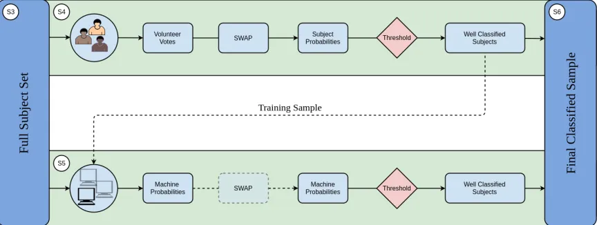
The Galaxy Zoo Express (GZX) framework combines human and machine to increase morphological classi-fication efficiency, both in terms of the classiclassi-fication rate and required human effort. Figure 1 presents a schematic of GZX including section numbers as a short-cut for the reader. We note that transparent portions of the schematic represent areas of future work which we explore in Section6. Any system combining human and machine classifications will have a set of generic fea-tures: a group of human classifiers, at least one machine classifier, and a decision engine which determines how these classifications should be combined.
In this work we demonstrate our system through a re-analysis of Galaxy Zoo 2 (GZ2) crowd-sourced classifi-cations as described in Section2. We compute “ground truth” labels for each galaxy in the GZ2 sample from the published GZ2 classification catalogue (Section2.1). The GZ2 data allow us to create simulations of human classifiers whose classifications are used most effec-tively when processed with SWAP, a Bayesian code first developed for the Space Warps gravitational lens dis-covery project (Marshall et al. 2016) and described in Section3. SWAP aggregates the crowd-sourced classifi-cations of galaxy images (hereafter,subjects) producing a final label for each subject (Section 3.3). We show that SWAP produces significant gains in classification efficiency as well as a reduction of human effort in Sec-tions3.4and3.5. In Section3.6we compare these labels to the “ground truth” labels computed from GZ2’s tra-ditional crowd-sourced classification method. Subjects classified by SWAP then provide the machine’s training sample.
Human and machine morphology classifications
Figure 1. Schematic of our hybrid system. Humans provide classifications of galaxy images via a web interface. We simulate this with the Galaxy Zoo 2 classification data described in Section 2. Human classifications are processed with an algorithm described in Section3. Subjects that pass a set of thresholds are considered human-retired (fully classified) and provide the training sample for the machine classifier as described in Section 4. The trained machine is applied to all subjects not yet retired. Those that pass an analogous set of machine-specific thresholds are considered machine-retired. The rest remain in the system to be classified by either human or machine. This procedure is repeated nightly. Our results are reported in Section5.
top-level question of the GZ2 decision tree, discussed below. Section4.4 discusses the decision engine we de-velop that delegates tasks between human classification and the Random Forest. After a sufficient number of subjects have been classified by humans via SWAP, the machine is trained and its performance assessed through cross-validation. This procedure is repeated nightly and the machine’s performance increases with the size of the training sample, albeit with a performance limit. Once the machine reaches an acceptable level of performance it is applied to the remaining galaxy sample as explored in Section4.5.
The results of our combined GZX system are provided in Section5. Even with this simple description, one can see that the classification process will progress in three phases. First, the machine will not yet have reached an acceptable level of performance; only humans contribute to subject classification. Second, the machine’s perfor-mance will improve; both humans and machine will be responsible for classification. Finally, machine perfor-mance will slow; remaining images will likely need to be classified by humans. This result is detailed in Section 5.1. Furthermore, in Section 5.2, we find evidence that the Random Forest may be capable of correctly identify-ing subjects that humans miss provididentify-ing a complimen-tary approach to galaxy classification. This blueprint allows even modest machine learning routines to make significant contributions alongside human classifiers and removes the need for ever-increasing performance in ma-chine classification. Discussion and conclusions are pre-sented in Section6.
2. GALAXY ZOO 2 CLASSIFICATION DATA
Our simulations utilize original classifications made by volunteers during the GZ2 project. These data1are
de-scribed in detail inWillett et al.(2013), though we pro-vide a brief overview here. The GZ2 subject sample con-sists of 285,962 galaxies identified as the brightest 25% (r-band magnitude < 17) residing in the SDSS North Galactic Cap region from Data Release 7 and included subjects with both spectroscopic and photometric red-shifts out to z < 0.25. Subjects were shown as colour composite images via a web-based interface2 wherein volunteers answered a series of questions pertaining to the morphology of the subject. With the exception of the first question, subsequent queries were dependent on volunteer responses from the previous task creating a complex decision tree3. Using GZ2 nomenclature, a
classificationis the total amount of information about a subject obtained by completing all tasks in the decision tree. A subject isretiredafter it has achieved a sufficient number of classifications.
For our current analysis, we choose the first task in the tree: “Is the galaxy simply smooth and rounded, with no sign of a disk?” to which possible responses include “smooth”, “features or disk”, or “star or artifact”. This choice serves two purposes: 1) this is one of only two questions in the GZ2 decision tree that is asked about every subject thus maximizing the amount of data we have to work with, and 2) our analysis assumes a binary task and this question is simple enough to cast as such.
1data.galaxyzoo.org 2
www.galaxyzoo.org
3 A visualization of this decision tree can be found athttps:
Specifically, we combine “star or artifact” responses with “features or disk” responses.
2.1. “Ground truth” labels
We assign each subject a descriptive label in order to validate our classification output against that of GZ2. GZ2 classifications are composed of volunteer vote frac-tions for each response to every task in the decision tree, denoted as fresponse. The most basic of these is com-puted simply asfr=nr/nt, that is, the number of votes of response r divided by the total number of votes for task t. Vote fractions are thus approximately contin-uous. A common technique is to place a threshold on these vote fractions to select samples with an empha-sis on purity or completeness, depending on the science case. For our current analysis we choose a threshold of 0.5, that is, if ffeatured+fartifact > fsmooth, the galaxy is labelled ‘Featured’, otherwise it is labelled ‘Not’. We note that only 512 subjects in the GZ2 catalogue have a majority fartifact, contributing less than half a per-cent contamination when combining the “star or arti-fact” with “features or disk” responses.
The GZ2 catalogue publishes three types of vote frac-tions for each subject: raw, weighted, and debiased. De-biased vote fractions are calculated to correct for red-shift bias, a task that GZX does not perform. The weighted vote fractions account for inconsistent volun-teers. The SWAP algorithm (described below) also has a mechanism to weight volunteer votes, however, the two methods are in stark contrast. For consistency, we thus derive labels from the simple “raw” vote frac-tions defined above, and designate the resulting labels as GZ2raw. In total, the data consist of over 14 million classifications from 83,943 individual volunteers.
The GZ2raw labels we compute from GZ2 vote frac-tions are used solely to validate our classification method and are thus considered “ground truth,” though this is, of course, subjective. Furthermore, we envision our framework being applied to never-before-classified image sets for which “ground truth” labels would not yet ex-ist. Nevertheless, in AppendixAwe show how different choices of our descriptive GZ2 labels change the per-ceived quality of our classification system and demon-strate that our method yields robust galaxy classifica-tions.
3. EFFICIENCY THROUGH INTELLIGENT HUMAN-VOTE AGGREGATION
Galaxy Zoo 2 did not have a predictive retirement rule, rather each galaxy received a median of 44 indepen-dent classifications. Once the project reached comple-tion, inconsistent volunteers were down-weighted ( Wil-lett et al. 2013), a process that does not make efficient use of those who are exceptionally skilled. To
intelli-gently manage subject retirement and increase classifi-cation efficiency, we adapt an algorithm from the Zooni-verse project Space Warps (Marshall et al. 2016), which searched for and discovered several gravitational lens candidates in the CFHT Legacy Survey (More et al. 2016). Dubbed SWAP (Space Warps Analysis Pipeline), this algorithm computed the probability that an image contained a gravitational lens given volunteers’ classifi-cations and experience after being shown a training sam-ple consisting of simulated lensing events. We provide an overview here; interested readers are encouraged to refer toMarshall et al.(2016) for additional details.
3.1. The SWAP algorithm
SWAP evaluates the accuracy of individual classifiers based on their responses to subjects where the true clas-sification is known, and applies those evaluations to the consensus classifications of subjects where the true clas-sification is unknown in order to improve clasclas-sification efficiency and reduce the classification effort required to complete a project. In order to achieve this, SWAP as-signs each volunteer anagent which interprets that vol-unteer’s classifications. Each agent assigns a 2×2 con-fusion matrix to their volunteer which encodes that vol-unteer’s probability to correctly identify featureAgiven that the subject exhibits feature A; and the probabil-ity to correctly identify the absence of feature A (de-notedN) given that the subject does not exhibit that feature. The agent updates these probabilities by esti-mating them as
P(“X”|X,d)≈ N“X” NX
(1)
whereXis the true classification of the subject and “X” is the classification made by the volunteer upon viewing the subject. ThusN“X” is the number of classifications the volunteer labelled as type X, NX is the number of subjects the volunteer has seen that were actually of typeX, and d represents the history of the volunteer, i.e., all subjects they have seen. Therefore the confusion matrix for a single volunteer goes as
M=
P(“A”|N,d) P(“A”|A,d)
P(“N”|N,d) P(“N”|A,d)
(2)
where probabilities are normalised such that
P(“A”|A) = 1−P(“N”|A).
Human and machine morphology classifications
0.0 0.2 0.4 0.6 0.8 1.0
P('Featured'|Featured)
0.0 0.2 0.4 0.6 0.8 1.0
P('Not'|Not)
"Obtuse"
"Pessimistic"
[image:5.612.53.296.61.303.2]"Optimistic"
"Astute"
"Random classifier"
Figure 2. Confusion matrices for 1000 randomly selected GZ2 volunteers after fiducial SWAP assessment. Circle size is proportional to the number of gold standard subjects each volunteer classified. The histograms on top and right repre-sent the distribution of each component of the confusion ma-trix for all volunteers. A quarter of GZ2 volunteers are “As-tute”: they correctly identify both ‘Featured’ and ‘Not’ sub-jects more than 50% of the time. The peaks at 0.5 in both distributions are due primarily to volunteers who see only one training image: only half of their confusion matrix is updated.
probability is updated after every volunteer classifica-tion, nudged higher or lower depending on volunteer in-put. Upper and lower probability thresholds can be set such that when a subject’s posterior crosses the upper threshold it is highly likely to exhibit featureA; while if it crosses the lower threshold it is highly likely that fea-tureAis absent. Subjects whose posteriors cross either of these thresholds are considered retired.
3.2. Gold-standard sample
A key feature of the original Space Warps project was the training of individual volunteers through the use of simulated images. These were interspersed with real imaging and were predominantly shown at the beginning of a volunteer’s engagement with the project, allowing that volunteer’s agent time to update before classifying real data. Volunteers were provided feedback in the form of a pop-up comment after classifying a training image. GZ2 did not train volunteers in such a way, presenting a challenge when applying SWAP to GZ2 classifications. Though we cannot retroactively train GZ2 volunteers, we develop a gold standard sample and arrange the or-der of gold standard classifications in oror-der to mimic the Space Warps system.
10
010
1No. of Classifications
10
210
110
0Posterior Probability P(Featured|
d
)
0
5
10
15
20
No
. o
f S
ub
jec
ts [
10
3
]
Non Gold Standard (GS)
GS: Featured
[image:5.612.326.555.62.421.2]GS: Not
Figure 3. Posterior probabilities for GZ2 subjects. The top panel depicts the probability trajectories of 200 randomly selected GZ2 subjects. All subjects begin with a prior of 0.5 denoted by the arrow. Each subject’s probability is nudged back and forth with each volunteer classification. From left to right the dotted vertical lines show the ‘Not’ threshold, prior probability, and ‘Featured’ threshold. Different colours denote different types of subjects. The bottom panel shows the distribution in probability for all GZ2 subjects by the end of our simulation, where the y axis is truncated to show detail.
We create a gold standard sample by selecting 3496 SDSS galaxies representative of the relative abundance of T-Types, a numerical index of a galaxy’s stage along the Hubble sequence, at z ∼ 0 by considering galax-ies that overlap with theNair & Abraham (2010) cat-alogue, a collection of ∼14K galaxies classified by eye into T-Types. We generate new expert labels for these galaxies that are consistent with the labels we defined for GZ2 classifications. These are provided by 15 pro-fessional astronomers, including members of the Galaxy Zoo science team, through the Zooniverse platform.4
4 The Project Builder template facility can be found athttp:
The question posed was identical to the original top-level GZ2 question and at least five experts classified each galaxy. Votes are aggregated and a simple ma-jority provides an expert label for each subject. This ensures that our expert labels are defined in exactly the same manner as the labels we assign the rest of the GZ2 sample. Our final dataset consists of the GZ2 classifica-tions made by those volunteers who classify at least one of these gold standard subjects. We thus retain for our simulation 12,686,170 classifications from 30,894 unique volunteers. When running SWAP, classifications of gold standard subjects are always processed first.
3.3. Fiducial SWAP simulation
Before we run a simulation, a number of SWAP pa-rameters must be chosen: the initial confusion matrix for each volunteer’s agent, (P(“F”|F),P(“N”|N)); the subject prior probability,p0; and the retirement thresh-olds, tF and tN. For our fiducial simulation we ini-tialize all confusion matrices at (0.5, 0.5), and set the subject prior probability, p0 = 0.5. We set the ‘Fea-tured’ threshold,tF, i.e., the minimum probability for a subject to be retired as ‘Featured’, to 0.99. Similarly, we set the ‘Not’ threshold, tN = 0.004. In AppendixBwe show that varying these parameters has only a small af-fect on the SWAP output. To simulate a live project, we run SWAP on a time step of ∆t= 1 day, during which SWAP processes all volunteer classifications with times-tamps within that range. This is performed for three months worth of GZ2 classification data. Hereafter, we refer to this asGZ2 project timewhere 0 marks the first day of the original GZ2 project.
[image:6.612.327.555.64.223.2]Figure 2 (adapted from Figure 4 of Marshall et al. 2016) demonstrates the volunteer assessment we achieve at the end of our simulation, and shows confusion ma-trices for 1000 randomly selected volunteers. The circle size is proportional to the number of gold standard sub-jects each volunteer classified. If we were to examine this figure immediately prior to the start of classifica-tions, it would show all points as small circles stacked precisely at the center of the figure since each volunteer is initially assigned a confusion matrix of (0.5, 0.5). As the simulation progresses, each volunteer’s green circle is updated in both location and size according to their as-sessment of gold standard subjects until arriving at the figure shown here. The histograms represent the distri-bution of each component of the confusion matrix for all volunteers. Nearly 25% of volunteers are considered “Astute” indicating they correctly identify both ‘Fea-tured’ and ‘Not’ subjects more than 50% of the time. Furthermore, as long as a volunteer’s confusion matrix is different from a random classifier, they provide use-ful information to the project. The spikes at 0.5 in the histograms are due to volunteers who see only one gold
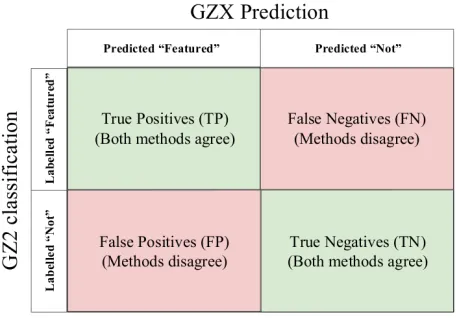
Figure 4. Confusion matrix for comparing our method to GZ2 which we consider to be “ground truth” as discussed in Section2.1. True positives (TP) and true negatives (TN) indicate that the predictions from our method agree with GZ2 for subjects labelled ‘Featured’ and ‘Not’, respectively. When the two classification methods disagree, the result is a sample of false negatives (FN) and false positives (FP). This allows us to easily compute quality metrics like accuracy, completeness, and purity with respect to GZ2 as shown in Equations3.
standard subject (i.e., ‘Featured’), leaving their proba-bility in the other (‘Not’) unchanged. Additionally, 4% of volunteers have a confusion matrix of (0.5, 0.5) indi-cating these volunteers classified two gold standard sub-jects of the same type, one correctly and one incorrectly. Figure 3 (adapted from Figure 5 of Marshall et al. 2016) demonstrates how subject posterior probabilities are updated with each classification. The arrow in the top panel denotes the prior probability,p0 = 0.5. With each classification, that prior is updated into a posterior probability creating a trajectory through probability space for each subject. The blue and orange lines show the trajectories of a random sample of ‘Featured’ and ‘Not’ subjects from our gold standard sample, while the black lines show the trajectories of a random sample of GZ2 subjects that were not part of the gold standard sample. The blue and orange dashed lines correspond to the retirement thresholds,tF andtN. The lower panel shows the full distribution of GZ2 subject posteriors at the end of our simulation, where the y-axis has been truncated to show detail. An overwhelming majority of subjects cross one of these retirement thresholds: of all subjects that SWAP “sees”, i.e., processes at least one classification, only 8% have not reached retirement by the end of our simulation.
Human and machine morphology classifications
explored in Section3.4). In contrast, a subject is consid-ered SWAP-retired once its posterior probability crosses either of the retirement thresholds defined above.
However, it is important not to prioritize efficiency at the expense of quality. Because we have a binary classi-fication, we can construct a confusion matrix from which we can compute the quality metrics of accuracy, com-pleteness and purity as a function of GZ2 project time by comparing our predicted labels to the GZ2rawlabels. Figure 4 graphically ascribes semantic interpretations for the elements of this confusion matrix. From these we compute:
accuracy = T P +T N
T P +F P +T N+F N
completeness = T P
T P +F N (3)
purity = T P
T P +F P
Thus a 100% complete sample recovers all subjects labelled ‘Featured’ by GZ2, whereas a 100% pure sample recovers only subjects labelled ‘Featured’ by GZ2. For example, by Day 20, SWAP retires 120K subjects with 96% accuracy, 99.7% completeness, and 92% purity.
Figure 5 and Table 1 detail the results of our fidu-cial SWAP simulation (“SWAP only”) compared to the original GZ2 project. The bottom panel shows the cu-mulative number of retired subjects as a function of GZ2 project time. By the end of our simulation, GZ2 (dashed dark blue) retires ∼50K subjects while SWAP (solid light blue) retires 226,124 subjects. We thus clas-sify 80% of the entire GZ2 sample in three months. Pro-cessing volunteer classifications through SWAP presents nearly a factor of 5 increase in classification efficiency. The top panel of Figure 5 demonstrates the quality of those classifications as a function of time and establishes that our full SWAP-retired sample is 95.7% accurate, 99% complete, and 86.7% pure. We discuss these small discrepancies in Section3.6.
3.4. Intelligent subject retirement
That SWAP achieves a classification rate nearly 5 times faster than GZ2 comes with a caveat: we consider only the top-level question of the GZ2 decision tree. It can be argued that GZ2 did not need∼40 votes per sub-ject to achieve exquisite sampling for the top-level ques-tion but rather adequate sampling for the subqueries. It might therefore be the case that the top-level question could be accurately resolved with far fewer classifica-tions. In order to put SWAP and GZ2 on equal footing we determine the minimum number of votes,N, that the GZ2 project would need in order to replicate the origi-nal GZ2 outcome for the top-level classification task for
0 20 40 60 80
Days in GZ2 Project
060 120 180 240
Cu
mu
lat
ive
re
tire
d s
ub
jec
ts [
10
3
]
SWAP
GZ2
0.750.80 0.85 0.90 0.95 1.00
Proportion
[image:7.612.323.559.60.400.2]Accuracy
Completeness
Purity
Figure 5. Fiducial SWAP simulation demonstrates a factor of 4.7 increase in the rate of subject retirement as a function of GZ2 project time (bottom panel, light blue) compared with the original GZ2 project (dashed dark blue). After 92 days, SWAP retires over 226K subjects, while GZ2 retires
∼48K. The top panel displays the quality metrics (greys). These are calculated by comparing labels predicted by SWAP to GZ2raw labels (Section 2) for the subject sample retired
by that day of the simulation. Thus, on the final day, SWAP retires 226,124 subjects with 95.7% accuracy, and with com-pleteness and purity of ‘Featured’ subjects at 99% and 86.7% respectively. The decrease in purity as a function of time is due, in part, to the fact that more difficult to classify subjects are retired later in the simulation (see Section3.4).
a canonical 95% of its sample.
We compute the raw vote fractions (ffeatured,fsmooth, and fartifact) for every subject in the GZ2 sam-ple using only the first N classifications for N ∈
[image:7.612.84.293.231.305.2]SWAP
10
15
20
25
30
35
GZ2 retirement at N votes
0.0
0.2
0.4
0.6
0.8
1.0
Fra
cti
on
of
vo
tes
at
N
=3
5
0.90
0.92
0.94
0.96
Accuracy
0.0
0.2
0.4
0.6
0.8
1.0
f
smooth0
5000
10000
15000
20000
Counts
All GZ2
SWAP retired
SWAP not (yet) retired
0
20
40
60
80
Votes at retirement
0.00
0.02
0.04
0.06
0.08
0.10
0.12
Normalized units
[image:8.612.62.545.70.391.2]Simulation: SWAP retired
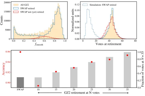
Figure 6. SWAP’s intelligent retirement mechanism requires only 30% of the classifications that GZ2 needs for the top-level question due to SWAP’s ability to retire easier subjects quickly, while more difficult subjects remain in the system to accrue additional classifications. Top panels: The top left panel showsfsmoothfor the entire GZ2 sample (orange), the subjects retired
by SWAP (blue), and subjects that SWAP has not yet retired by the end of our simulation (red). The latter distribution peaks at fsmooth ∼0.6, which can intuitively be understood as the most difficult to classify subjects: those withfsmooth ≤0.5 are
easily identified as ‘Featured’, while those withfsmooth≥0.8 are more obviously ‘Not’. The top right panel provides additional
evidence showing the number of votes at retirement for both the original GZ2 project (solid lines) and our SWAP simulation (dashed blue). The left-skew inherent in the red SWAP-not-yet-retired sample is due to difficult-to-classify subjects that received only 30-40 classifications during the GZ2 project. Even after processing all available classifications, SWAP cannot retire these subjects without additional volunteer input. Bottom panel: Here we compare SWAP to results of simulations of GZ2 run with a lower retirement limit in order to evaluate whether or not GZ2’s considerable number of votes per subject are necessary solely to populate subqueries. Solid bars show the number of classifications required to retire the same number of galaxies as SWAP (dark grey) for different fixed retirement limits in GZ2 (light grey). The height of the bars are normalised to show the counts relative to the highest simulated GZ2 retirement limit we test (N= 35, right vertical axis). The accuracy of the classifications for these simulated GZ2 runs against the full GZ2 project are shown as red points (left vertical axis). If GZ2 retirement were set at a level (N = 10) that reproduces the total number of classifications logged by SWAP, the accuracy would be below 90% (versus SWAP’s 96%). Instead, GZ2 requires, at minimum, 3.5 times as many votes to approach the same accuracy (95%) as SWAP. Simulated GZ2 sessions were run 100 times, randomly selecting subsamples with the same number of galaxies as were retired during our fiducial SWAP simulation. Quantities shown are averages of these trials; statistical error bars are too small to be seen.
order to achieve consistent class labels 95% of the time, a full 3.5 times more classifications than SWAP needs to achieve the same accuracy. Furthermore, this justifies our choice of defining a subject as GZ2-retired once it reaches at least 30 classifications.
SWAP’s performance can be explained through its tirement mechanism. GZ2 did not have a predictive re-tirement rule, rather the project was declared complete when the median classification count for the ensemble reached a value that was deemed to be sufficient for
Human and machine morphology classifications
0 10 20 30 40 50 60
Classifications till retirement
0.00 0.02 0.04 0.06 0.08 0.10 0.12
Frequency
[image:9.612.59.296.66.236.2]All Retired 'Not' 'Featured' Fixed : 'Not' Fixed : 'Featured'
Figure 7. SWAP’s volunteer-weighting mechanism provides a factor of three reduction in the human effort required to retire GZ2 subjects. The filled histograms show the num-ber of volunteer classifications per subject achieved during our SWAP simulation broken down by class label, where the solid black line is the total. The dashed histograms are results from our toy model in which we simulate volun-teers with fixed confusion matrices, effectively disengaging SWAP’s volunteer-weighting mechanism. These broad dis-tributions require ∼3 times more classifications per subject to reach the same retirement thresholds.
SWAP-retired sample generally follows the same distri-bution as GZ2-full except for the noticeable dip around
fsmooth= 0.6. In contrast, the SWAP-not-yet-retired sample peaks atfsmooth= 0.6. These subjects can be in-terpreted as being the most difficult to classify which can be understood intuitively: galaxies with fsmooth ≤ 0.5 are easily identified as having features, while galaxies withfsmooth ≥0.8 are more obviously elliptical.
This is further corroborated in the top right panel of Figure6 which shows the distribution of the number of classifications a subject had at the time of retirement. The solid lines show this distribution from the original GZ2 project for the same subsamples as the top left panel. For comparison, the dashed line shows the num-ber of classifications at retirement realized during our SWAP simulation. Again, we see that the SWAP-retired sample is representative of GZ2 as a whole. However, the distribution for the SWAP-not-yet-retired sample is skewed toward fewer total classifications.
To understand this, consider the following: GZ2 served subject images at random with the exception that, towards the end of the project, subjects with low numbers of classifications were shown at a higher rate (Willett et al. 2013). The median number of classifica-tions was 44 with the full distribution shown in orange in the top right panel of Figure6. Our SWAP simulation processes these classifications in the same order as the original project (with the exception that gold-standard subject classifications are processed first as described
in Section 3.2). Because our simulations cycle through only 92 days of GZ2 data, there are three general scenar-ios for why a subject has not yet been retired through SWAP: 1) SWAP has seen only a few of the many clas-sifications for a given subject and it is not yet enough to retire it, 2) SWAP has seen many of the classifications for a subject but that subject is difficult; if we ran the simulation longer to process the remaining GZ2 classifi-cations, SWAP would eventually retire it, and 3) SWAP has seen most or all of the classifications for a subject but it is difficult and there are few or no remaining GZ2 classifications; without additional volunteer input, these subjects will never be retired by SWAP.
It is this third category that skews the red distribution towards fewer GZ2 votes. These are difficult-to-classify subjects that have only 30 - 40 GZ2 classifications, all of which are processed by SWAP, but these subjects re-main unretired. This is an indication that such subjects should have continued to accrue classifications in order to reach strong consensus.
We have demonstrated that SWAP retires subjects intelligently: quickly retiring easy-to-classify subjects while allowing those that are more difficult to collect ad-ditional classifications. SWAP thus requires only 30% of the votes that GZ2 needs and retires nearly 5 times as many subjects during the three months of GZ2 project time that we include in our simulation.
3.5. Reducing human effort
SWAP’s intelligent retirement mechanism is charac-terised, in large part, by the way SWAP estimates vol-unteer classification ability. This in turn allows for a dra-matic reduction in the amount of human effort (votes) required. To see this more clearly, we consider a toy model wherein we simulate volunteers with fixed con-fusion matrices. We simulate 1000 ‘Featured’ subjects and 1000 ‘Not’ subjects each with prior, p0 = 0.5. We simulate 100 volunteer agents all with the same fixed confusion matrix of (0.63, 0.65), where these values are computed as the averageP(“F”|F) andP(“N”|N) from our assessment of real volunteers, excluding the spikes at 0.5. We generate volunteer classifications based on this confusion matrix (i.e., volunteers will correctly iden-tify ‘Featured’ subjects 63% of the time) and update the subject’s posterior probability with each classifica-tion. We track how many classifications are required for each subject’s posterior to cross either the ‘Featured’ or ‘Not’ retirement thresholds.
0.0
0.2
0.4
0.6
0.8
1.0
GZ2
f
features+
f
artifact0.00
0.05
0.10
0.15
0.20
0.25
0.30
Proportion
Correct
[image:10.612.62.295.64.252.2]False Positives ×10
False Negatives ×100
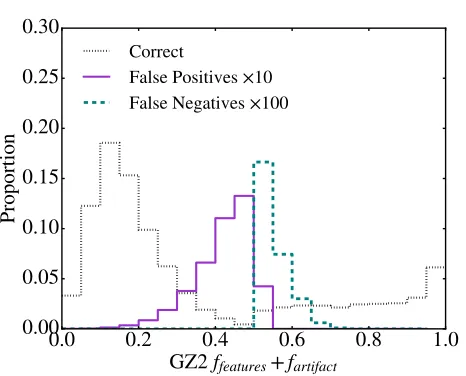
Figure 8. Distribution of GZ2 ffeatured+fartifact vote
frac-tions for subjects correctly identified by SWAP (dotted grey), along with those identified as false positives (solid purple), and false negatives (dashed teal). The false positives and false negatives are scaled by factors of 10 and 100 respec-tively for easier comparison. From Section2, subjects with values>0.5 are defined as ‘Featured’, however, the teal dis-tribution indicates that SWAP labels them as ‘Not’. This is not necessarily a flaw of SWAP: 68.9% of incorrectly identi-fied subjects have 0.4≤ffeatured+fartifact ≤0.6, nearly the
same range as a 68% confidence interval around our choosen threshold. The overlap between the false positives and neg-atives is due to subjects that are exactly 50-50; by default these are labelled ‘Not’.
for volunteer ability, most subjects are retired with be-tween 6 and 15 votes, with a median of 9 votes. In contrast, when every volunteer is given equal weight-ing, subjects require 16 to 45 votes with a median of 30 votes before crossing one of the retirement thresh-olds. Thus the volunteer weighting scheme embedded in SWAP can reduce the amount of human effort required to retire subjects by a factor of three.
This reduction will be, in part, a function of the num-ber of gold standard subjects each volunteer sees. Our gold standard sample was chosen to be representative of morphology rather than evenly distributed among GZ2 volunteers. We thus find that half of our volunteers clas-sify only one or two gold standard subjects. That we achieve a factor of three reduction when only half of our volunteer pool has seen≥2 gold standard subjects suggests that an additional reduction of human effort is possible with more extensive volunteer training.
3.6. Disagreements between SWAP and GZ2
Galaxy Zoo’s strength comes from the consensus of dozens of volunteers voting on each subject. Process-ing votes with SWAP reduces the number of classifica-tions to reach consensus. Though we typically recover the GZ2rawlabel, SWAP disagrees about 5% of the time.
We thus examine the false positives (subjects SWAP la-bels as ‘Featured’ but GZ2raw labels as ‘Not’) and false negatives (subjects SWAP labels as ‘Not’ but GZ2raw la-bels as ‘Featured’). We explore these subjects in red-shift, magnitude, physical size, and concentration but find no correlation with any of these variables, suggest-ing that, at least for this galaxy sample, the reliability of morphology depends on factors that are not captured by these coarse measurements. This is perhaps unsurpris-ing since GZ2 subjects were selected from the larger GZ1 sample to be the brightest, largest and nearest galaxies: precisely those subjects most accessible for visual clas-sification.
Instead we consider the stochastic nature of GZ2 vote fractions, which can be estimated as binomial. Let suc-cess be a response of “smooth” and failure be any other response. The 68% confidence interval on a subject with
fsmooth = 0.5 is then (0.42,0.57) assuming 40 classifica-tions, each with a probability of 0.5. Figure 8 shows the distribution of ffeatured+fartifact for the false pos-itives (solid purple), and the false negatives (dashed teal) compared to the subjects where SWAP and GZ2 agree (dotted grey). Recall that if this value is greater than 0.5, the subject is labelled ‘Featured’. The ma-jority of disagreements between SWAP and GZ2 are for subjects that have 0.4 < ffeatured+fartifact <0.6. It is thus unsurprising that SWAP and GZ2 disagree most within the approximate confidence interval of our se-lected GZ2 threshold. We note that the distribution overlap between false positives and false negatives is due to subjects that do not have a majority; these are la-belled ‘Not’ by default.
Two other effects contribute to the disagreement be-tween SWAP and GZ2. First, as the number of clas-sifications used to retire a galaxy decreases, the likeli-hood of misclassification by random chance increases. Second, disagreement arises due to expert-level volun-teers whose confusion matrices are close to 1.0. These volunteers are essentially more strongly weighted, allow-ing that subject’s posterior to cross a retirement thresh-old in as few as two classifications. In rare cases, de-spite training, some expert-level volunteers get it wrong compared to the gold-standard labels. These issues can be mitigated by requiring each subject reach a mini-mum number of classifications in addition to its pos-terior probability crossing a retirement threshold, thus combining the best qualities of GZ2 and SWAP.
3.7. Summary
Human and machine morphology classifications
purity that can be controlled by careful selection of in-put parameters to be better than 90% (see AppendixB). Exploring those subjects wherein SWAP and GZ2 dis-agree, we conclude that the majority of this disagree-ment stems from the stochastic nature of GZ2raw la-bels. We now turn our focus towards incorporating a machine classifier utilizing these SWAP-retired subjects as a training sample.
4. EFFICIENCY THROUGH INCORPORATION OF MACHINE CLASSIFIERS
We construct the full Galaxy Zoo Express by incor-porating supervised learning, the machine learning task of inference from labelled training data. The training data consist of a set of training examples, and must include an input feature vector and a desired output la-bel. Generally speaking, a supervised learning algorithm analyses the training data and produces a function that can be mapped to new examples. A properly optimized algorithm will correctly determine class labels for un-seen data. By processing human classifications through SWAP, we obtain a set of binary labels by which we can train a machine classifier. We briefly outline the tech-nical details of our machine below, turning towards the decision engine we develop in Section4.4.
4.1. Random Forests
We use a Random Forest (RF) algorithm (Breiman 2001), an ensemble classifier that operates by boot-strapping the training data and constructing a multi-tude of individual decision tree algorithms, one for each subsample. An individual decision tree works by de-ciding which of the input features best separates the classes. It does this by performing splits on the val-ues of the input feature that minimize the classifica-tion error. These feature splits proceed recursively. Decision trees alone are prone to over-fitting, preclud-ing them from generalispreclud-ing well to new data. Random Forests mitigate this effect by combining the output la-bels from a multitude of decision trees. Specifically, we use the RandomForestClassifierfrom the Python modulescikit-learn(Pedregosa et al. 2011).
4.2. Grid Search and Cross-validation
Of fundamental importance is the task of choos-ing an algorithm’s hyperparameters, values which de-termine how the machine learns. For a RF, key quantities include the maximum depth of individual trees (max depth), the number of trees in the forest (n estimators), and the number of features to con-sider when looking for the best split (max features). The goal is to determine which values will optimize the machine’s performance and thus these values can-not be chosena priori. We perform a grid search with
k-fold cross-validation whereby the training sample is split into k subsamples. One subsample is withheld to estimate the machine’s performance while the remaining data are used to train the machine. This is performed
ktimes and the average performance value is recorded. The entire process is repeated for every combination of the hyperparameters in the grid space and values that optimize the output are chosen. In this work we let
k = 10, however, we leave this as an adjustable input parameter. In the interest of computational speed, we setn estimators= 30 and perform the grid search for
max depthover the range [5,16], andmax featuresover the range [√D, D], where D is the number of features in the feature vector, described below.
4.3. Feature Representation and Pre-Processing
The feature vector on which the machine learns is composed ofDindividual numeric quantities associated with the subject that the machine uses to discern that subject from others in the training sample. To segre-gate ‘Featured’ from ‘Not’, we draw on ZEST ( Scar-lata et al. 2007) and compute concentration, asymme-try, Gini coefficient, and M20, the second-order moment of light for the brightest 20% of galaxy pixels, as mea-sured from SDSS DR12 i-band imaging (see Appendix C). Coupled with SExtractor’s measurement of elliptic-ity (Bertin & Arnouts 1996), we provide the machine with aD= 5 dimensional morphology parameter space. These non-parametric diagnostics have long been used to distinguish between early- and late-type galaxies in an automated fashion (e.g.,Abraham et al. 1996;Bershady et al. 2000;Conselice et al. 2000; Abraham et al. 2003; Conselice 2003;Lotz et al. 2004;Snyder et al. 2015). Be-cause the RF algorithm handles a variety of input for-mats, the only pprocessing step we perform is the re-moval of poorly-measured morphological indicators, i.e. catastrophic failures.
4.4. Decision Engine
A number of decisions must be addressed before at-tempting to train the machine. In particular, which subjects should be designated as the training sample? When should the machine attempt its first training ses-sion? When has the machine’s performance been opti-mized such that it will successfully generalize to unseen subjects? The field of machine learning provides few hard rules for answering these questions, only guidelines and best practices. Here we briefly discuss our approach for the development of our decision engine.
ei-0
10
20
30
40
Training sample size [10
3]
0.75
0.80
0.85
0.90
0.95
1.00
Accuracy
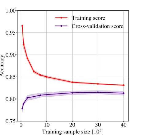
[image:12.612.52.283.73.293.2]Training score
Cross-validation score
Figure 9. Learning curve for a Random Forest with fixed hyperparameters. These curves show the mean accuracy computed during cross-validation and on the training sam-ple, where the shaded regions denote the standard deviation. When the training sample size is small, the machine accu-rately identifies its own training sample but is unable to gen-eralize to unseen data as evidenced by a low cross-validation score. This score increases with the size of the training sam-ple but eventually plateaus indicating that larger training samples provide little in additional performance.
ther of the retirement thresholds. Though we find that SWAP consistently retires 35-40% ‘Featured’ subjects on any given day of the simulation, a balanced ratio of ‘Featured’ to ‘Not’ isn’t guaranteed. Highly unbal-anced training samples should be resampled to correct the imbalance; however, as we exhibit only a mild lop-sidedness, we allow the machine to train on all SWAP-retired subjects.
SWAP retires a few hundred subjects during the first days of the simulation. In principle, a machine can be trained with such a small sample, but will be unable to generalize to unseen data. We estimate a minimum number of training samples and the machine’s ability to generalize by considering a learning curve, an illustra-tion of a machine’s performance with increasing sample size for fixed hyperparameters. Figure 9 demonstrates such a curve wherein we plot the accuracy from both the 10-fold cross-validation, and the trained machine ap-plied to its own training sample for a random sample of GZ2 subjects required to be balanced between ‘Fea-tured’ and ‘Not’. We fix the RF’s hyperparameters as follows: max depth = 8, n estimators = 30, and
max features= 2. When the sample size is small, the cross-validation score is low and the training score is high, a clear sign of over-fitting. However, as the traing sample size increases, the cross-validation score
in-creases and eventually plateaus, indicating that larger training sets will yield little additional gain.
We estimate this plateau begins when the training sample reaches 10,000 subjects and require SWAP re-tire at least this many before the machine attempts its first training. We estimate the machine has trained suf-ficiently if the cross-validation score fluctuates by less than 1% for three consecutive nights of training to en-sure we have reached the plateau. This requires that we record the machine’s training performance each night, including how well it scores on the training sample, the cross-validation score, and the best hyperparameters.
4.5. The Machine Shop
We can now describe a full GZX simulation, which begins with human classifications processed through SWAP for several days. Once at least 10K subjects have been retired, their feature vectors are passed to the machine for its inaugural training. A suite of per-formance metrics are recorded by a machine agent, sim-ilar in construction to SWAP’s agents. This agent de-termines when the machine has trained sufficiently by assessing the variation in performance metrics for all previous nights of training. Once the machine has been optimized, the agent introduces it to the test sample consisting of any subject that has not yet reached retire-ment through SWAP and is not part of the gold standard sample.
Analogous to SWAP, we generate a retirement rule for machine-classified subjects. In addition to the class pre-diction, the RF algorithm computes the probability for each subject to belong to each class. This probability is simply the average of the probabilities of each individ-ual decision tree, where the probability of a single tree is determined as the fraction of subjects of class X on a leaf node. Only subjects that receive a class predic-tion of ‘Featured’ with pmachine ≥ 0.9 (pmachine ≤ 0.1 for ‘Not’) are considered retired. The remaining sub-jects have the possibility of being classified by humans or the machine on a future night of the simulation. This constitutes the core of our passive feedback mechanism. Subjects that are not retired by the machine can in-stead be retired by humans, thus providing the machine a more fully sampled morphology parameter space on future training sessions.
5. RESULTS
Human and machine morphology classifications
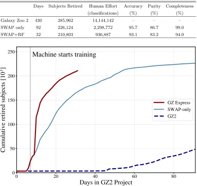
Table 1. Summary of key quantities for GZ2 and our various simulations. All quality metrics are calculated using GZ2rawlabels.
Simulation Summary
Days Subjects Retired Human Effort Accuracy Purity Completeness
(classifications) (%) (%) (%)
Galaxy Zoo 2 430 285,962 14,144,142 – – –
SWAP only 92 226,124 2,298,772 95.7 86.7 99.0
SWAP+RF 32 210,803 936,887 93.1 83.2 94.0
0
20
40
60
80
Days in GZ2 Project
0
50
100
150
200
250
Cu
mu
lat
ive
re
tire
d s
ub
jec
ts [
10
3
]
Machine starts training
GZ Express
SWAP-only
GZ2
Figure 10. By incorporating a machine classifier, GZX (red) increases the classification rate by an order of magnitude compared to GZ2 (dashed dark blue) and out-performs the SWAP-only run (light blue), retiring more than 200K subjects in just 27 days of GZ2 project time. The dashed black line marks the first night the machine trains. After several additional nights of training, it is deemed optimized and allowed to retire subjects. Both humans and machine then contribute to retirement. We end the simulation after 32 days having retired over 210K galaxies. See Table1for details.
has deemed the machine optimized. The machine pre-dicts class labels for the remaining 230K GZ2 subjects. Of those, the machine retires over 70K, dramatically increasing the subset of retired subjects. We end the simulation after 32 days, having retired∼210K subjects as detailed in Table1.
We present these results in Figure10 where subject retirement with GZX (red) is compared to our fidu-cial SWAP-only run (light blue) and GZ2 (dashed dark blue). Using the GZ2raw labels as before, we compute our usual quality metrics on the full sample of GZX-retired subjects; reported in Table1. Accuracy and pu-rity remain within a few percent of the SWAP-only run at 93.1% and 83.2% respectively. Instead we see a 5% decline in the completeness. While the SWAP-only run identified 99% of ‘Featured’ subjects, incorporation of
the machine seems to miss a significant portion thus dropping GZX completeness to 94.0%. We discuss this behaviour below.
0 5 10 15 20 25 30
Days in GZ2 Project
0 50 100 150 200 250
Cu
mu
lat
ive
re
tire
d s
ub
jec
ts [
10
3
]
GZX: SWAP+RF GZX: RF GZX: SWAP SWAP-only
0 10 20 30
Days in GZ2 project
0.0 0.1 0.2 0.3 0.4 0.5 0.6 0.7
Fraction
Featured
0 10 20 30
[image:14.612.55.291.54.432.2]Days in GZ2 project
Not Featured
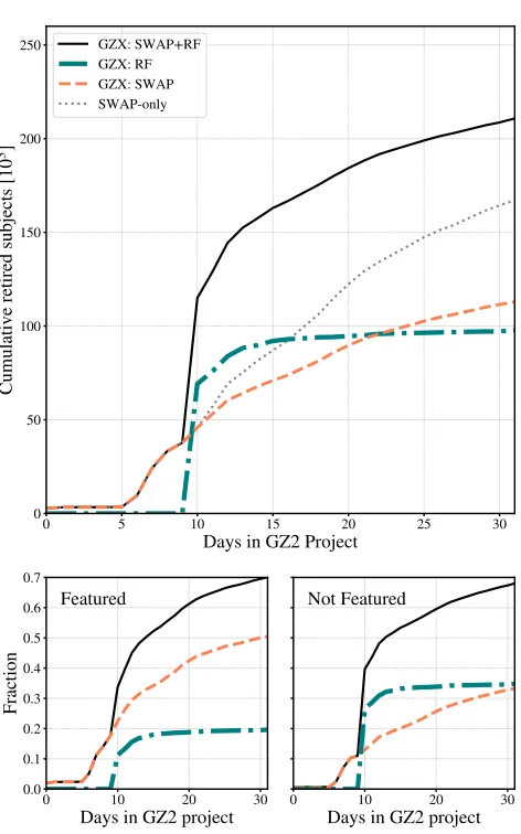
Figure 11. Contributions to subject retirement by both clas-sifying agents of GZX: human (SWAP, orange) and machine (RF, teal). The top panel shows cumulative subject retire-ment for GZX as a whole (solid black), along with that at-tributed to the RF and SWAP. The dotted grey line shows the fiducial SWAP-only run for comparison. Retirement to-tals for humans and machine are nearly equal over the course of the simulation but display different behaviours: SWAP’s retirement rate is almost constant while the RF contributes substantially after its initial application and then plateaus. The bottom panels show what fraction of GZ2 subjects are retired, separated by class label. Overall, GZX retires 73.7% of the entire GZ2 sample in 32 days, retiring the same propor-tion of ‘Featured’ and ‘Not’ subjects as indicated by the black lines. However, humans retire 30% more ‘Featured’ subjects than the machine, while both components retire a similar proportion of ‘Not’ subjects.
5.1. Who retires what, when?
In the top panel of Figure 11 we explore the indi-vidual contributions to GZX subject retirement from the RF (dash-dotted teal) and SWAP (dashed orange). The solid black line shows the total GZX retirement (SWAP+RF), while the dotted grey line depicts the fiducial SWAP-only run from Section 3.3 for reference. Two things are immediately obvious. First, each compo-nent shoulders approximately half of the retirement
bur-den with the machine and SWAP responsible for∼98K and∼112K subjects respectively. Secondly, the rate of retirement exhibited by the two components is in stark contrast. SWAP retires at a relatively constant rate while the machine retires dramatically at the beginning of its application, quickly surpassing the human con-tribution, and plateaus thereafter. We thus clearly see three epochs of subject retirement. In the first phase, humans are the only contributors to subject retirement. Once the machine is optimized, it immediately con-tributes more to retirement than humans. However, the machine’s performance plateaus quickly; the third phase is again dominated by human classifications.
In the bottom panels of Figure 11, we consider the class composition of subjects retired by SWAP and the RF. The left (right) panel shows the retired fraction of GZ2 subjects identified as ‘Featured’ (‘Not’) accord-ing to their GZ2raw labels as a function of GZ2 project time. Overall, GZX retires 73.7% of the GZ2 sub-ject sample and this is evenly distributed between ‘Fea-tured’ and ‘Not’ subjects as indicated by the solid black lines in both panels. However, SWAP retires more than 50% of all ‘Featured’ subjects while the machine retires only 20%. This divergence does not exist for ‘Not’ sub-jects where each component contributes 33-34%.
What is the source of this discrepancy? Each night the machine trains on a sample composed consistently of 30-40% ‘Featured’ subjects but does not retire a similar proportion, indicating that the 30% of non-retired ‘Fea-tured’ subjects do not receive highpmachine. In the fol-lowing section we explore whether this is an artefact of our choice in machine or in the human-machine combi-nation implemented here.
5.2. Machine performance
Throughout our analysis we have defined ‘Fea-tured’ and ‘Not’ subjects by their GZ2raw labels as this was the most compatible choice for comparison with SWAP output. However, the machine does not learn in the same way, nor is it presented with the same infor-mation. Machine and human classifications each provide valuable and complementary information for identifying ‘Featured’ galaxies.
We isolate the 7060 subjects that were deemed false positives, i.e., galaxies retired by the machine as ‘Fea-tured’ that have ‘Not’ GZ2rawlabels, a sample that com-prises only 7.2% of all subjects the machine retires. We visually examine several hundred and assess that, to the expert eye, a majority are, in fact, ‘Featured’. A random sample is shown in Figure12.
Human and machine morphology classifications
Figure 12. A random subsample of subjects identified as false positives: labelled by machine as ‘Featured’ but as ‘Not’ according to GZ2raw. We displayffeaturedin the lower left corner, that is, the fraction of volunteers who classified the subject as ‘Featured’.
Values are typically under 0.35 indicating that GZ2 volunteers strongly believed these to be ‘smooth’ (‘Not’). Fortunately, the machine is able to identify these subjects as ‘Featured’ due to their measured morphology diagnostics.
0.4 0.5 0.6 0.7 0.8
G
Normalized Distribution
1.5 2.0 2.5
M20 2 3 C 4 5 0.2 0.4 0.6 0.81 b/a 0.05 0.15 A 0.25 0.35
All subjects 'Not' 'Featured'
Figure 13. The RF is trained on a 5-dimensional morphology parameter space. We show the distribution of each morphology indicator for machine-retired ‘Featured’ (blue) and ‘Not’ (orange) subjects compared to the full GZ2 subject sample (black). The difference between ‘Featured’ and ‘Not’ subjects is in stark contrast for all distributions except, perhaps,M20.
we chose carries with it a confidence interval such that subjects with 0.4 < ffeatured+fartifact < 0.6 are most likely to receive disagreeing labels from other classify-ing agents, 2) the first task of the GZ2 decision tree asks a question that does not necessarily correlate with a split between early- and late-type galaxies, and 3) the machine learns on morphology diagnostics that are very different from visual inspection.
We find that 40% of these false positives have 0.4 ≤ ffeatured+fartifact< 0.5 indicating that the dis-agreement between humans and machine is likely due to the labels we assign at our given threshold.
How-ever, we also find that 45% of false positives have
[image:15.612.58.559.400.529.2]M20 1 b/a C A G 0.0
0.1 0.2 0.3 0.4
[image:16.612.54.280.56.226.2]Feature Importance
Figure 14. The RF’s ranked feature importance averaged over all nights of training with black bars indicating the stan-dard deviation. A larger value corresponds to higher impor-tance. The machine computes feature importance according to how much each feature increases the purity of the result-ing split averaged over all trees in the forest. The RF places great importance in the Gini coefficient though we note that it can under-represent the importance of highly correlated features such as concentration.
particular question, if either human or machine iden-tifies a subject as ‘Featured’, it is likely the subject is discy and worth further investigation.
Accordingly, this suggests that, in some cases, the morphology indicators we measure are sufficient for the machine to recognize ‘Featured’ galaxies regardless of the labels humans provide. Figure 13shows the distri-bution of each morphology indicator for all subjects the machine retires as ‘Featured’ (blue) and ‘Not’ (orange) compared to the full GZ2 subject set. The difference between ‘Featured’ and ‘Not’ is stark in all but theM20 distribution. This can be seen explicitly in Figure 14 in which we show the RF’s ranked feature importances, where large values indicate higher importance. Feature importance is computed as how much each feature de-creases the impurity of a split in a tree. The impurity decrease from each feature is then averaged over all trees and ranked. We show the feature importance averaged over all nights of training with black bars indicating the standard deviation. The machine finds the Gini coeffi-cient most important for class prediction, placing little emphasis onM20. It is well known that the Gini coef-ficient is more sensitive to noise than other diagnostics, however, we point out that when a machine is faced with two or more correlated features any of them can be used as the predictor. Once chosen, the importance of the others is reduced. This explains why Concentra-tion is ranked much lower than Gini even though they are strongly correlated as seen in Figure B3. That the machine relies heavily on these two morphology diag-nostics is unsurprising as concentration has long been an automated predictor between early- and late-type
galax-ies (Abraham et al. 1994, 1996; Shen et al. 2003). The complementary nature of human and machine classification can best be utilized by a feedback mech-anism in which a portion of machine-retired subjects are reviewed by humans. Subjects that display exces-sive disagreement should be verified by an expert (or expert-user). In the same way that humans increase the machine’s training sample over time, subjects that the machine properly identifies can become part of the hu-mans’ training sample.
6. LOOKING FORWARD
We have demonstrated the first practical framework for combining human and machine intelligence in galaxy morphology classification tasks. While we focus below on a brief discussion of our next steps and potential applications to large upcoming surveys, we note that our results have implications for the future of citizen science and Galaxy Zoo in particular.
GZX is perhaps one of the simplest ways to combine human and machine intelligence and its impressive per-formance motivates a higher level of sophistication. A first step will be an implementation of SWAP that can handle a complex decision tree. In addition, we envision multiple forms of active feedback in addition to our pas-sive feedback mechanism. SWAP allows us to leverage the most skilled volunteers to review galaxies difficult for either human or machine to classify. Additionally, machine-retired subjects should contribute to the train-ing sample for humans in an analogous fashion to what we have already implemented.
Secondly, our RF can be improved by providing it in-formation equal to what humans receive: multi-band morphology diagnostics will be included in our future feature vector. However, the Random Forest algorithm is not easily adapted to handle measurement errors or class labels with continuous distributions. A key feature of GZ2 vote fractions is their use in determining the strength of a a morphological feature. Although both SWAP and our RF provide class predictions that are continuous, we apply thresholds to discretize the classi-fication. To fully utilize the information provided, so-phisticated algorithms should be considered such as deep convolutional neural networks (CNN) or Latent Dirich-let allocation (LDA), an algorithm that is frequently used in document processing. Furthermore, there is no reason to limit to a single machine. As hinted at in Fig-ure1, several machines could train simultaneously, their predictions aggregated through SWAP, creating an on-the-fly machine ensemble.
Human and machine morphology classifications
surveys. By some estimates, Euclid is expected to ob-tain measurable morphology with its visual instrument (VIS) for approximately 106
−107 galaxies (Laureijs
et al. 2011). Visual classification at the rate achieved with Galaxy Zoo today would require 12–120 years to classify.5 If theEuclid sample is on the high end, GZX
as currently implemented could classify the brightest 20% during the six years of its observing mission. As currently implemented, we obtain accuracy around 95% potentially leaving hundreds of thousands of galaxies with unreliable classifications. In a companion paper that seeks to identify supernovae, Wright et al. (2017) demonstrate a dramatic increase in accuracy through an entirely different human-machine combination whereby the scores from human and machine are averaged to-gether with the combined score yielding the most reli-able classification. Again, a combination of both ap-proaches will allow us to take full advantage of legacy output from large scale surveys.
6.1. Conclusions
In this paper we design and test Galaxy Zoo Express, an innovative system6for the efficient classification of
galaxy morphology tasks that integrates the native abil-ity of the human mind to identify the abstract and novel with machine learning algorithms that provide speed and brute force. We demonstrate for the first time that the SWAP algorithm, originally developed to identify rare gravitational lenses in the Space Warps project, is robust for use in galaxy morphology classification. We show that by implementing SWAP on GZ2 classification data we can increase the rate of classification by a fac-tor of 4-5, requiring only 90 days of GZ2 project time to classify nearly 80% of the entire galaxy sample.
Furthermore, we have implemented and tested a Ran-dom Forest algorithm and developed a decision engine that delegates tasks between human and machine. We show that even this simple machine is capable of pro-viding significant gains in the classification rate when combined with human classifiers: GZX retires over 70% of GZ2 galaxies in just 32 days of GZ2 project time. This represents a factor of at least 8 increase in the classification rate as well as nearly an order of magni-tude reduction in human effort compared to the orig-inal GZ2 project. This is achieved without sacrificing the quality of classifications as we maintain∼94% accu-racy throughout our simulations. Additionally, we have shown that training on a 5-dimensional parameter space
of traditional non-parametric morphology indicators al-lows the machine to identify subjects that humans miss, providing a complementary approach to visual classifica-tion. The gain in classification speed allows us to tackle the massive amount of data promised from large surveys likeLSST andEuclid.
We are grateful to the anonymous referees for help-ful comments and suggestions which greatly improved this manuscript. MB thanks Steven Bamford and Boris H¨außler for insightful discussions on citizen science and Galaxy Zoo; and John Wallin and Marc Huertas-Company for several enlightening conversations on ma-chine learning and classification. We are grateful to Elisabeth Baeten, Micaela Bagley, Karlen Shahinyan, Vihang Mehta, Steven Bamford, Kevin Schawinski, and Rebecca Smethurst for providing expert classifications in addition to those provided by the authors. PJM acknowledges Aprajita Verma and Anupreeta More for their ongoing collaboration on the Space Warps project. MB, CS, LF, KW, and MG gratefully acknowledge partial support from the US National Science Foun-dation (NSF) Grant AST-1413610. LF and DW also gratefully acknowledge partial support from NSF IIS 1619177. MB acknowledges additional support through New College and Oxford University’s Balzan Fellowship as well as the University of Minnesota Doctoral Dis-sertation Fellowship. Travel funding was supplied to MB, in part, by the University of Minnesota Thesis Re-search Travel Grant. CJL recognizes support from a grant from the Science & Technology Facilities Coun-cil (ST/N003179/1). BDS acknowledges support from Balliol College, Oxford, and the National Aeronautics and Space Administration (NASA) through Einstein Postdoctoral Fellowship Award Number PF5-160143 is-sued by the Chandra X-ray Observatory Center, which is operated by the Smithsonian Astrophysical Observa-tory for and on behalf of NASA under contract NAS8-03060. The work of PJM is supported by the U.S. De-partment of Energy under contract number DE-AC02-76SF00515. This publication uses data generated via the Zooniverse.org platform, development of which is funded by generous support, including a Global Impact Award from Google, and by a grant from the Alfred P. Sloan Foundation.
Software:
scikit-learn (Pedregosa et al. 2011),As-tropy (Astropy Collaboration et al. 2013), TOPCAT (Taylor 2005)
5We note that the classification rate of GZ2 was 4 times higher
than GZ’s current steady rate.
6Our code can be found athttps://github.com/melaniebeck/