http://www.scirp.org/journal/ojbm ISSN Online: 2329-3292
ISSN Print: 2329-3284
DOI: 10.4236/ojbm.2018.62025 Apr. 25, 2018 349 Open Journal of Business and Management
Research on State Transition Model Based on
Stock Market Volume-Price Distribution
Yin Tang, Muxing Lin
Management School, Jinan University, Guangzhou, China
Abstract
This paper discusses Volume-Price distribution of stock market. The normal distribution-like structures spanning different time are studied, based on which we propose a predictive model of Volume-Price distribution in China stock market. The paper includes three parts: First, the hypothesis that the Chinese stock market day trading volume-price distributions does not obey normal distribution is verified. However, a “fat tail” approximate normal dis-tribution pattern is founded. After smoothing the disdis-tribution of volume and price, approximate normal distributions of trading volume and price distribu-tions for different time spans are discovered. On the basis of two previous studies, state transition model of volume-price distributions is proposed. State transition probability table is created based on clustering analysis. The mode can appropriately account for the transition Chinese stock market trading vo-lume-price distribution network transitions between states, and can be used to predict possible future distribution, to provide a quantitative indicator in the stock market investment.
Keywords
Time Series, State Transition, Volume-Price Distribution
1. Introduction
Due to chaos in financial market, traditional financial engineering, which is typ-ically based on econometrics method with linear assumption and casualty, usually does not work out. Most of regression models, neglect rich cross section information of financial time series, and try to predict specific price, which is nearly impossible. Models with low loss data reduction on rich cross section in-formation become a challenge for researchers.
This paper first examines the hypothesis whether the distribution of volume How to cite this paper: Tang, Y. and Lin,
M.X. (2018) Research on State Transition Model Based on Stock Market Volume-Price Distribution. Open Journal of Business and Management, 6, 349-361.
https://doi.org/10.4236/ojbm.2018.62025
Received: March 21, 2018 Accepted: April 22, 2018 Published: April 25, 2018
Copyright © 2018 by authors and Scientific Research Publishing Inc. This work is licensed under the Creative Commons Attribution International License (CC BY 4.0).
DOI: 10.4236/ojbm.2018.62025 350 Open Journal of Business and Management and price is subject to a certain probability distribution, and then the discrete-ness of distribution transition over time. Based on the above hypotheses, it is possible to predict the distribution of future prices, and form investment strate-gies. Therefore, the research is based on a large number of micro-data to study the distribution of the micro-structure of volume-price distributions, and the approximate simplification of normal distribution. On the basis of scale-free microstructure, a state transition model is proposed to describe the evolution of dynamic equilibrium of financial market. The micro-structure of financial mar-ket and the dynamic transition between each state are explored, and the quantit-ative suggestions and guidance for the investment behavior of financial market are put forward.
2. Literature Review
Clark [1] believes that the volume of transactions is positively related to the vo-latility of prices, and proposes a preliminary model of the mixed distribution hypothesis (MDH), assuming that information will cause simultaneous changes in price volatility and volume. Based on this, Epps and Epps [2] examined the mechanism of intraday trading through theoretical and empirical models, and considered that market heterogeneity, absolute price change, and volume have a certain positive correlation, and the change in price logarithm obeys the transac-tion. The quantity is a mixed distribution of mixed variables, and the mixed dis-tribution has a higher kurtosis. Tauchea and Pitts [3] extended the hybrid dis-tribution hypothesis theory to derive joint probability disdis-tributions and volume of price changes for any time interval of intraday trading from economic theory, and based on how more and more traders enter (or exit). The market is to de-termine the changes in the joint distribution. Harris (1982) [4] [5][6] pointed out that the mixed distribution hypothesis can explain the “thick tail” characte-ristics of daily price changes, as well as the positive correlation between earnings volatility and trading volume. These studies assume the probability distribution of price changes, but do not provide a model for the evolution of probability distribution over time.
DOI: 10.4236/ojbm.2018.62025 351 Open Journal of Business and Management the market to provide liquidity for arbitrage [13]. Serge Darolles, Gaëlle Le Fol, and Gulten Mero [14] included information flow and liquidity shocks in the re-lationship between volatility and volume. Some studies of developing country markets also support mixed distribution hypotheses [15] [16] [17]. Therefore, the impact of the information flow on the probability and distribution of the quantity and price as well as the impact results requires further analysis.
Wu Chongfeng and Wu Wenfeng [18] integrated the time dimension, trans-action price, and trading volume, and used a simple segmentation function to reconstruct the stock price series based on volume using the dimensional trans-formation. The GARCH model was used to demonstrate the feasibility. Zhang Yongyi et al. [19] used a regression model to study the dynamic relationship between historical volume price information and price information. The empir-ical results showed that trading volume information is more conducive to price discovery than historical price information. Li Mengxuan and Zhou Yi [20] used the Granger causality test to study the relationship between high-frequency trading stock market prices and trading volume. Chen Qiling and Song Fengm-ing [21] used econometric models to examine the correlation between price changes and trading volumes in the Chinese stock market. The empirical results all point out that the absolute value of daily trading price volatility in the Chi-nese stock market is directly proportional to the trading volume, and this corre-lation is not symmetrical. Li Shuangcheng [22] used the asymmetric GARCH-M model to find that the hybrid distribution hypothesis was also established in Shanghai and Shenzhen cities in China. The Shanghai stock market responded more quickly to the transaction volume as an alternative indicator of informa-tion flow.
All in all, the above study found the probability distribution of price changes, but it did not consider the volume. On the other hand, the evolution of the probability distribution still lacks applicable models.
3. State Transition Model of Volume-Price Distribution
Definition 1. Volume-Price Distribution. The stock market is an ever-changing time series, choosing a time series as a segment, the prices of all transactions in the segment and their corresponding total transactions constitute a distribution function that describes the functional relationship between the price and the vo-lume in the transaction time series within segment of the stock market.Definition 2. State of Volume-Price Distribution. The parameters (mean and variance, for instance) to describe the Volume-Price Distribution, is considered as a state. Different time series segments of different clusters belong to different states.
DOI: 10.4236/ojbm.2018.62025 352 Open Journal of Business and Management The idea is, first to propose an algorithm to fit the normal distribution to Vo-lume-Price distribution. Secondly, we use the exhaustive method and the genetic algorithm to optimize the search. We search for the approximate micro-structure of the normal distribution in the data training set, and calculate the correspond-ing parameters; then cluster the above microscopic structure, use the endogen-ous and exogenendogen-ous method to calculate the optimal cluster structure, and estab-lish the state transition table between states based on the original state transition data. Finally, a state transition model based on dynamic equilibrium is estab-lished according to the parameters, and the correctness of the state transition model is verified with the verification set data.
Assumption. Volume-price distribution transits between different states with a certain probability. This assumes the distribution has discrete states, which will be verified by clustering techniques in the following sections.
State Clustering Algorithm. Using k-mean clustering method, 9000 state time intervals are divided into K clusters, among which the number of cluster K is determined by combining the endogenous method and the exogenous me-thod. Based on previous empirical experience, we select sqrt (n/2) as the number of clusters k, then the expected number of elements per cluster is sqrt (2 × n).
State Transition Probability Algorithm. The algorithm sorts the segmented intervals of the approximate normal distribution pattern by time, and generates the transition probability before different states. The state transition matrix is established based on the time series statistics of the state transitions: Calculate the total number of possible states after each state transition in the time series, and divide the total number of occurrences of each state by the total number as the transition probability between the two states, and establish a state transition matrix.
Construction of State Transition Models
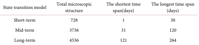
The Construction of short-, medium-, and long-term state transition models are shown in Table 1.
Short-term state transition model: To establish a short-term state transition model, we acquire approximately normal distribution within time span no more than 30 days, from the 1st to the 695th microscopic structures. The KMEANS clustering method is used to analyze the approximate normal distribution struc-ture morphology (K = 19), and the state transition table calculated (Table 2). Based on the short-term state transition table in Table 2, predict four successive normal distributions. The expected value of prediction is 0.82, and the probabil-ity of correct prediction is 0.20.
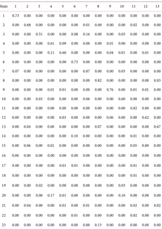
Mid-term state transition model: likewise, time span is greater than 30 days and less than or equal to 90 days, data from 1st to 3700th microscopic structures. The KMEANS coefficient K = 43 (Table 3). The predicted expected value is 1.40, and the predicted correct probability 0.35.
DOI: 10.4236/ojbm.2018.62025 353 Open Journal of Business and Management
Table 1. Construction of short-, medium-, and long-term state transition models.
State transition model Total microscopic structure The shortest time span(days) The longest time span (days)
Short-term 728 1 30
Mid-term 3736 31 120
Long-term 4536 121 264
Source: composed by authors.
Table 2. Short-term state transition table.
State 1 2 3 4 5 6 7 8 9 10 11 12 13 14 15 16 17 18 19 1 0.48 0.05 0.02 0.00 0.05 0.00 0.02 0.02 0.02 0.18 0.00 0.05 0.00 0.00 0.00 0.02 0.00 0.09 0.00 2 0.00 0.20 0.00 0.00 0.00 0.20 0.00 0.00 0.00 0.00 0.00 0.00 0.00 0.00 0.20 0.00 0.00 0.40 0.00 3 0.00 0.00 0.50 0.15 0.00 0.00 0.00 0.00 0.10 0.00 0.00 0.00 0.10 0.00 0.00 0.05 0.00 0.05 0.05 4 0.14 0.00 0.03 0.27 0.14 0.03 0.19 0.00 0.00 0.05 0.11 0.00 0.00 0.00 0.00 0.00 0.00 0.00 0.05 5 0.08 0.00 0.00 0.15 0.38 0.00 0.08 0.00 0.00 0.00 0.08 0.15 0.00 0.00 0.00 0.00 0.00 0.08 0.00 6 0.05 0.00 0.00 0.11 0.00 0.53 0.11 0.11 0.00 0.00 0.00 0.00 0.00 0.00 0.00 0.00 0.05 0.05 0.00 7 0.09 0.00 0.02 0.16 0.02 0.02 0.23 0.05 0.02 0.00 0.05 0.05 0.00 0.06 0.00 0.05 0.00 0.18 0.02 8 0.00 0.00 0.00 0.07 0.00 0.00 0.02 0.39 0.10 0.10 0.00 0.00 0.00 0.02 0.02 0.12 0.00 0.12 0.02 9 0.00 0.00 0.11 0.00 0.00 0.00 0.00 0.07 0.46 0.04 0.00 0.00 0.00 0.00 0.00 0.07 0.00 0.25 0.00 10 0.06 0.00 0.00 0.00 0.03 0.00 0.13 0.05 0.00 0.62 0.00 0.02 0.00 0.02 0.02 0.03 0.00 0.02 0.02 11 0.00 0.00 0.00 0.00 0.00 0.60 0.00 0.00 0.00 0.00 0.20 0.00 0.20 0.00 0.00 0.00 0.00 0.00 0.00 12 0.14 0.04 0.00 0.11 0.07 0.00 0.07 0.00 0.00 0.04 0.00 0.36 0.00 0.00 0.04 0.11 0.00 0.00 0.04 13 0.00 0.00 0.09 0.00 0.00 0.05 0.00 0.00 0.00 0.00 0.05 0.00 0.64 0.00 0.00 0.09 0.00 0.09 0.00 14 0.00 0.08 0.00 0.00 0.00 0.00 0.08 0.00 0.00 0.00 0.04 0.00 0.00 0.24 0.20 0.04 0.12 0.04 0.16 15 0.00 0.00 0.00 0.00 0.00 0.00 0.06 0.00 0.06 0.06 0.00 0.00 0.00 0.12 0.47 0.00 0.00 0.18 0.06 16 0.00 0.04 0.00 0.00 0.04 0.00 0.00 0.08 0.04 0.00 0.00 0.00 0.04 0.08 0.04 0.44 0.00 0.04 0.16 17 0.00 0.00 0.00 0.00 0.00 0.00 0.33 0.33 0.00 0.00 0.00 0.00 0.00 0.00 0.00 0.00 0.33 0.00 0.00 18 0.03 0.00 0.00 0.07 0.00 0.04 0.10 0.09 0.07 0.00 0.01 0.00 0.00 0.00 0.00 0.01 0.00 0.54 0.01 19 0.00 0.00 0.13 0.00 0.00 0.07 0.00 0.03 0.00 0.00 0.00 0.00 0.03 0.10 0.00 0.03 0.00 0.03 0.57
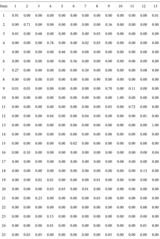
K = 42 (Table 4). The expected value is 2 and the expected probability of correct prediction 0.5.
DOI: 10.4236/ojbm.2018.62025 354 Open Journal of Business and Management
Table 3. Mid-term state transition table.
State 1 2 3 4 5 6 7 8 9 10 11 12 13
1 0.73 0.00 0.00 0.00 0.00 0.00 0.00 0.00 0.00 0.00 0.00 0.00 0.00 2 0.00 0.68 0.00 0.00 0.00 0.00 0.01 0.00 0.00 0.00 0.02 0.00 0.00 3 0.00 0.00 0.51 0.00 0.00 0.08 0.16 0.00 0.00 0.03 0.00 0.00 0.00 4 0.00 0.00 0.00 0.61 0.09 0.00 0.00 0.00 0.01 0.00 0.00 0.00 0.00 5 0.00 0.00 0.00 0.11 0.60 0.00 0.00 0.00 0.04 0.01 0.00 0.01 0.00 6 0.00 0.00 0.00 0.00 0.00 0.73 0.00 0.00 0.00 0.00 0.00 0.00 0.00 7 0.07 0.00 0.00 0.00 0.00 0.00 0.87 0.00 0.00 0.03 0.00 0.00 0.00 8 0.00 0.00 0.00 0.00 0.00 0.00 0.00 0.82 0.00 0.00 0.00 0.00 0.03 9 0.00 0.00 0.00 0.01 0.01 0.00 0.00 0.00 0.76 0.00 0.01 0.01 0.00 10 0.00 0.00 0.03 0.00 0.00 0.00 0.06 0.00 0.00 0.60 0.00 0.00 0.00 11 0.00 0.00 0.00 0.00 0.00 0.00 0.00 0.00 0.00 0.00 0.82 0.00 0.00 12 0.00 0.00 0.00 0.00 0.03 0.00 0.00 0.00 0.06 0.00 0.00 0.62 0.00 13 0.00 0.04 0.00 0.00 0.00 0.00 0.00 0.07 0.00 0.00 0.00 0.00 0.67 14 0.00 0.00 0.00 0.00 0.00 0.10 0.00 0.00 0.00 0.00 0.01 0.00 0.00
15 0.00 0.06 0.00 0.01 0.00 0.00 0.00 0.00 0.00 0.00 0.05 0.00 0.00
16 0.00 0.00 0.00 0.00 0.00 0.00 0.00 0.00 0.00 0.00 0.00 0.00 0.00
17 0.00 0.00 0.00 0.00 0.01 0.01 0.00 0.00 0.00 0.00 0.01 0.00 0.00
18 0.00 0.00 0.00 0.00 0.00 0.00 0.00 0.00 0.00 0.00 0.01 0.00 0.00
19 0.00 0.00 0.02 0.00 0.00 0.00 0.00 0.00 0.00 0.03 0.00 0.00 0.00
20 0.00 0.00 0.00 0.17 0.01 0.00 0.00 0.00 0.00 0.10 0.00 0.00 0.00
21 0.00 0.04 0.00 0.00 0.01 0.00 0.01 0.00 0.00 0.00 0.02 0.00 0.02
22 0.00 0.00 0.00 0.00 0.00 0.01 0.00 0.00 0.00 0.00 0.02 0.00 0.00 23 0.00 0.00 0.00 0.00 0.00 0.00 0.00 0.13 0.00 0.00 0.00 0.00 0.00
(Note: table shows partially due to large amount data).
the actual value the parameters describing the morphological structure of the approximate normal distribution are, the higher the accuracy of the model is.
4. Data and Experiments
DOI: 10.4236/ojbm.2018.62025 355 Open Journal of Business and Management
Table 4. Long-term state transition table.
State 1 2 3 4 5 6 7 8 9 10 11 12 13
1 0.91 0.00 0.00 0.00 0.00 0.00 0.00 0.00 0.00 0.00 0.00 0.00 0.01 2 0.00 0.71 0.00 0.00 0.00 0.00 0.00 0.00 0.16 0.00 0.00 0.00 0.00 3 0.01 0.00 0.68 0.00 0.00 0.00 0.00 0.03 0.00 0.00 0.00 0.00 0.00 4 0.00 0.00 0.00 0.76 0.00 0.00 0.02 0.03 0.00 0.00 0.00 0.00 0.00 5 0.00 0.00 0.00 0.00 0.66 0.00 0.00 0.00 0.00 0.00 0.00 0.00 0.00 6 0.00 0.00 0.00 0.00 0.06 0.56 0.00 0.00 0.00 0.00 0.00 0.00 0.00 7 0.27 0.00 0.00 0.00 0.00 0.00 0.50 0.00 0.00 0.00 0.00 0.08 0.00 8 0.00 0.00 0.00 0.05 0.00 0.00 0.00 0.90 0.00 0.00 0.00 0.00 0.00 9 0.01 0.05 0.00 0.00 0.00 0.00 0.00 0.00 0.70 0.00 0.11 0.00 0.00 10 0.00 0.00 0.00 0.00 0.00 0.00 0.00 0.00 0.00 1.00 0.00 0.00 0.00 11 0.00 0.00 0.00 0.00 0.00 0.00 0.00 0.00 0.05 0.00 0.72 0.00 0.00 12 0.00 0.00 0.00 0.04 0.00 0.00 0.04 0.00 0.00 0.00 0.00 0.81 0.00 13 0.00 0.00 0.00 0.00 0.00 0.00 0.00 0.00 0.00 0.00 0.00 0.00 1.00 14 0.00 0.00 0.00 0.00 0.00 0.00 0.00 0.00 0.00 0.00 0.00 0.00 0.00 15 0.00 0.00 0.00 0.00 0.00 0.02 0.00 0.00 0.00 0.00 0.00 0.00 0.00 16 0.00 0.10 0.00 0.00 0.00 0.00 0.00 0.00 0.00 0.00 0.00 0.00 0.04 17 0.00 0.00 0.00 0.00 0.00 0.00 0.00 0.00 0.00 0.08 0.00 0.00 0.00 18 0.00 0.00 0.00 0.00 0.00 0.00 0.00 0.00 0.00 0.00 0.00 0.13 0.00 19 0.00 0.00 0.02 0.01 0.00 0.00 0.00 0.01 0.00 0.00 0.00 0.00 0.00 20 0.00 0.00 0.00 0.03 0.03 0.00 0.01 0.00 0.00 0.00 0.00 0.00 0.00 21 0.00 0.00 0.23 0.00 0.00 0.00 0.00 0.03 0.00 0.00 0.00 0.00 0.00 22 0.00 0.00 0.00 0.00 0.00 0.00 0.00 0.00 0.00 0.00 0.00 0.00 0.00 23 0.00 0.00 0.00 0.15 0.00 0.00 0.00 0.00 0.00 0.00 0.00 0.00 0.00 24 0.00 0.00 0.00 0.01 0.00 0.00 0.00 0.00 0.00 0.00 0.00 0.01 0.00 25 0.00 0.03 0.05 0.00 0.00 0.00 0.00 0.00 0.05 0.00 0.00 0.00 0.00
(Note: table shows partially due to large amount data).
(SH000002) stock from June 1, 2007 to April 29, 2010 was selected as the basic research data.
DOI: 10.4236/ojbm.2018.62025 356 Open Journal of Business and Management density curve is fitted to the normal distribution, and parameters (mean and va-riance) obtained are described as the state of the segment.
This experiment investigates possible state transitions between time interval segments with a “normal peak-thick tail” approximate normal distribution pat-tern. By clustering approximate normal distribution structures and dividing them into different states. The frequency and probability of each state transition is calculated to construct a state transition probability matrix, which make poss-ible the future transition.
The idea is to establish a model on the short-term (with time span no more than one month), medium-term (with time span between 1 and 3 months), and long-term (with time span greater than 3 months). Experimental steps are as follows:
1) Cluster approximate normal distribution structure in each time interval. The K-MEANS method is used to cluster the mean and variance of the approx-imate morphology of normal distribution structure, 2 - 100 cluster clusters were calculated.
2) Select better clustering result (i.e., the corresponding number of clus-ters). Using three intrinsic methods (empirical method, elbow method, and cross-validation method), the cluster number set with better clustering effect is obtained.
3) Use external methods to determine the optimal clustering result (that is, the corresponding number of clusters). The correct predicted expected number of preferred cluster number sets is calculated, so that the highest expected number of correctly predicted clusters becomes the best.
4) According to clustering results, construct the state transition matrix. Clus-ter the original training set and the test set, and calculate the probability of tran-sitions between states, then form a state transition matrix to predict the future transitions.
5) Predict the possibility of a state transition of the verification set and calcu-late the transition prediction result. The established state transition model is ap-plied to verify the state transition of the set, and the probabilities are calculated.
4.1. Empirical Validation
Based on the state transition table, a state transition model is established, which can be used to determine the parameters describing the approximate normal structure of the future transaction volume price distribution—mean and va-riance. The mean value indicates the center of gravity of the future transaction price, that is, the price range of future larger transactions. The variance represents the concentration of future trading volume. The greater the variance, the lower the concentration, and the more the trading volume tends to be in the price region. The smaller the variance, the higher the concentration, whereas the trading volume tends to be concentrated in the area near the average value.
DOI: 10.4236/ojbm.2018.62025 357 Open Journal of Business and Management constructed with the approximate normal distribution micro-structure in time span within 30 days (Table 5). The mid-term and long term validation are omitted due to limit space of the paper.
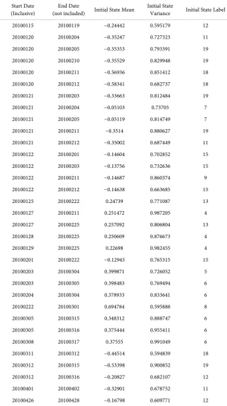
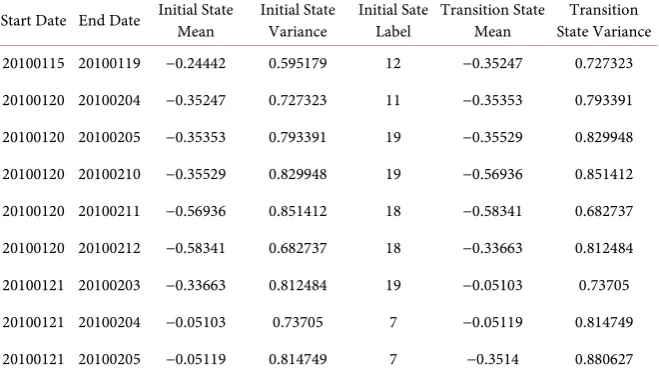
The 1st to 694th microscopic structures are chosen as training set to establish the state transition model, and the data between the 695th and 727th, total of 33 microstructures, are used as the validation set (Table 6).
4.2. Experiment Steps and Results
1) A short-term state transition model is established based on the training set, and a probability generator is constructed. The next state of the transition is predicted according to the input state;
2) According to each state in the model, the normal distribution description parameter range corresponding to each state is calculated (Table 7), and para-meter of the next state is randomly generated according;
3) Repeat step 1) and 2) for 200 times, then average the obtained parameter group as the parameter to predict the next state;
4) Quantify and compare the predicted normal distribution description with actual normal distribution description (Table 8).
5. Conclusions
In this paper, the discrete density distribution is continuously used by using the kernel density method. It is proposed and verified that there are a large number of scale-free approximate normal distribution morphological structures in the stock trading volume and price distribution. The state transition model con-structed can be applied to the volume and price distribution of stock trading is forecasted.
The main contribution of the paper is to cluster the nonstandard metric va-lence distribution structures according to different time spans of the approx-imate normal distribution morphological structure, establish a state transition model, determine the approximate normal distribution morphological structure of the range of parameters (mean and variance), and indicate the state Different accuracy and limitations of the transition model.
The limitations of this paper are as follows: 1) The state transition model de-signed and constructed in this paper centralizes the transaction price, has dem-onstrated its scale-free characteristics, and is conducive to the comparison and analysis of the approximate normal distribution morphological structure. How-ever, the model established in this paper can only determine the deviation be-tween the center of gravity and the center value, and cannot give a specific point
Table 5. Short-term state transition model data.
State transition model Total microscopic structure The shortest time span (days) The longest time span (days)
DOI: 10.4236/ojbm.2018.62025 358 Open Journal of Business and Management
Table 6. Validation sets.
Start Date
(Inclusive) (not included) End Date Initial State Mean Initial State Variance Initial State Label
20100115 20100119 −0.24442 0.595179 12
20100120 20100204 −0.35247 0.727323 11
20100120 20100205 −0.35353 0.793391 19
20100120 20100210 −0.35529 0.829948 19
20100120 20100211 −0.56936 0.851412 18
20100120 20100212 −0.58341 0.682737 18
20100121 20100203 −0.33663 0.812484 19
20100121 20100204 −0.05103 0.73705 7
20100121 20100205 −0.05119 0.814749 7
20100121 20100211 −0.3514 0.880627 19
20100121 20100212 −0.35002 0.687449 11
20100122 20100201 −0.14604 0.702852 15
20100122 20100203 −0.13756 0.732636 15
20100122 20100211 −0.14687 0.860374 9
20100122 20100212 −0.14638 0.663685 15
20100125 20100222 0.24739 0.771087 13
20100127 20100211 0.251472 0.987205 4
20100127 20100225 0.257092 0.806804 13
20100128 20100225 0.250609 0.876673 4
20100129 20100225 0.22698 0.982455 4
20100201 20100222 −0.12945 0.765315 15
20100203 20100304 0.399871 0.726052 5
20100203 20100305 0.398483 0.769494 6
20100204 20100304 0.378933 0.833641 6
20100222 20100301 0.694784 0.595888 8
20100305 20100315 0.348312 0.888747 6
20100305 20100316 0.375444 0.955411 6
20100308 20100317 0.37555 0.991049 6
20100311 20100312 −0.44514 0.594839 18
20100312 20100315 −0.53398 0.900852 19
20100312 20100316 −0.20827 0.682107 12
20100401 20100402 −0.32901 0.678752 11
20100426 20100428 −0.16798 0.609771 12
DOI: 10.4236/ojbm.2018.62025 359 Open Journal of Business and Management
Table 7. Characteristics of validation sets.
Start Time End Time Normal Distribution Description Mean Description Variance Normal Distribution Status
20100115 20100119 −0.2444226 0.5951795 12
20100120 20100204 −0.3524684 0.7273228 11
Table 8. Results of transition prediction.
Start Date End Date Initial State Mean Initial State Variance Initial Sate Label Transition State Mean State Variance Transition
20100115 20100119 −0.24442 0.595179 12 −0.35247 0.727323 20100120 20100204 −0.35247 0.727323 11 −0.35353 0.793391 20100120 20100205 −0.35353 0.793391 19 −0.35529 0.829948 20100120 20100210 −0.35529 0.829948 19 −0.56936 0.851412 20100120 20100211 −0.56936 0.851412 18 −0.58341 0.682737 20100120 20100212 −0.58341 0.682737 18 −0.33663 0.812484 20100121 20100203 −0.33663 0.812484 19 −0.05103 0.73705 20100121 20100204 −0.05103 0.73705 7 −0.05119 0.814749 20100121 20100205 −0.05119 0.814749 7 −0.3514 0.880627
price. It is helpful to compare and analyze the morphological structure of the approximate normal distribution, and neglect the comparison of the absolute value of the volume of each different approximate normal distribution morpho-logical structure, and cannot predict the future specific volume; 3) Financial time series. The segmentation problem also affects the prediction of specific time points and time spans of the future state.
Acknowledgements
This research is supported by Guangdong Province Applied Science and Tech-nology Research and Development Special Fund Project (2016B010124008), Guangdong Province Science and Technology Development Special Fund (2016B040401003), Guangdong Province Science and Technology Development Special Fund (2016A010101016).
References
[1] Clark, P.K. (1973) A Subordinated Stochastic Process Model with Finite Variance for Speculative Prices. Econometrica, 41, 135-155. https://doi.org/10.2307/1913889
[2] Epps, T.W. and Epps, M.L. (1976) The Stochastic Dependence of Security Price Changes and Transaction Volumes: Implications for the Mixture of Distributions Hypothesis. Econometrica, 44, 305-321. https://doi.org/10.2307/1912726
[3] Tauchen, G.E. and Pitts, M. (1983) The Price Variability-Volume Relationship on Speculative Markets. Econometrica, 51, 485-505. https://doi.org/10.2307/1912002
[image:11.595.210.540.180.369.2]Spe-DOI: 10.4236/ojbm.2018.62025 360 Open Journal of Business and Management
culative Prices and of the Relation between Absolute Price Change and Volume. Unpublished Ph.D. Dissertation, University of Chicago, Chicago.
[5] Harris, L. (1986) Cross-Security Tests of the Mixture of Distributions Hypothesis.
Journal of Financial & Quantitative Analysis, 21, 39-46.
https://doi.org/10.2307/2330989
[6] Harris, L. (1987) Transaction Data Tests of the Mixture of Distributions Hypothe-sis. Journal of Financial & Quantitative Analysis, 22, 127-141.
https://doi.org/10.2307/2330708
[7] Lamoureux, C.G. and Lastrapes, W.D. (1994) Endogenous Trading Volume and Momentum in Stock-Return Volatility. Journal of Business & Economic Statistics, 12, 253-260.
[8] Andersen, T.G. (1996) Return Volatility and Trading Volume: An Information Flow Interpretation of Stochastic Volatility. Journal of Finance, 51, 169-204.
https://doi.org/10.1111/j.1540-6261.1996.tb05206.x
[9] Amihud, Y. (2002) Illiquidity and Stock Returns: Cross-Section and Time-Series Effects. Journal of Financial Markets, 5, 31-56.
https://doi.org/10.1016/S1386-4181(01)00024-6
[10] Acharya, V.V. and Pedersen, L.H. (2005) Asset Pricing with Liquidity Risk. Social Science Electronic Publishing, 77, 375-410.
https://doi.org/10.1016/j.jfineco.2004.06.007
[11] Chordia, T., Roll, R. and Subrahmanyam, A. (2001) Market Liquidity and Trading Activity. Journal of Finance, 56, 501-530. https://doi.org/10.1111/0022-1082.00335
[12] Chordia, T., Subrahmanyam, A. and Anshuman, V.R. (2001) Trading Activity and Expected Stock Returns. Journal of Financial Economics, 59, 3-32.
https://doi.org/10.1016/S0304-405X(00)00080-5
[13] Darolles, S. and Fol, G.L. (2014) Trading Volume and Arbitrage. Working Papers. [14] Darolles, S., Fol, G.L. and Mero, G. (2008) When Market Illiquidity Generates
Vo-lume. Working Papers.
[15] Chong, S.P., Lee, S.Y. and Nam, K. (2000) Volatility and Information Flows in Emerging Equity Market: A Case of the Korean Stock Exchange. International Re-view of Financial Analysis, 9, 405-420.
https://doi.org/10.1016/S1057-5219(00)00037-5
[16] Ibrahim, I. and Othman, Y. (2000) The Relationship between Trading Volume, Re-turns and Volatility in the Kuala Lumpur Stock Exchange. Jurnal Pengurusan, 19. [17] Bohl, M.T. and Henke, H. (2003) Trading Volume and Stock Market Volatility: The
Polish Case. International Review of Financial Analysis, 12, 513-525.
https://doi.org/10.1016/S1057-5219(03)00066-8
[18] Wu, C. and Wu, W. (2001) Stock Price Sequence Analysis Based on Volume. Jour-nal of Systems Management, 10, 1-7. (In Chinese)
[19] Zhang, Y., Wang, C. and Hua, C. (2013) Is Historical Price Information More Effec-tive in Price Discovery?—Data Analysis Based on China’s Stock Market. Chinese Journal of Management Science, No. s1, 346-354. (In Chinese)
[20] Li, M. and Zhou, Y. (2009) Research on the Relationship between Volume and Price in China Stock Market Based on High Frequency Data. Statistics and Decision, No. 3, 132-133. (In Chinese)
DOI: 10.4236/ojbm.2018.62025 361 Open Journal of Business and Management Science, 3, 62-68. (In Chinese)