http://wrap.warwick.ac.uk
Original citation:
Li, Ang, Staunton, Richard and Tjahjadi, Tardi. (2013) Rational-operator-based depth-from-defocus approach to scene reconstruction. Journal of the Optical Society of America A: Optics, Image Science and Vision, Volume 30 (Number 9). pp. 1787-1795. ISSN 1084-7529
Permanent WRAP url:
http://wrap.warwick.ac.uk/56213
Copyright and reuse:
The Warwick Research Archive Portal (WRAP) makes this work by researchers of the University of Warwick available open access under the following conditions. Copyright © and all moral rights to the version of the paper presented here belong to the individual author(s) and/or other copyright owners. To the extent reasonable and practicable the material made available in WRAP has been checked for eligibility before being made available.
Copies of full items can be used for personal research or study, educational, or not-for-profit purposes without prior permission or charge. Provided that the authors, title and full bibliographic details are credited, a hyperlink and/or URL is given for the original metadata page and the content is not changed in any way.
Publisher’s statement:
This paper was published in Journal of the Optical Society of America A: Optics, Image Science and Vision and is made available as an electronic reprint with the permission of OSA. The paper can be found at the following URL on the OSA website:
http://dx.doi.org/10.1364/JOSAA.30.001787 . Systematic or multiple reproduction or distribution to multiple locations via electronic or other means is prohibited and is subject to penalties under law.
A note on versions:
The version presented here may differ from the published version or, version of record, if you wish to cite this item you are advised to consult the publisher’s version. Please see the ‘permanent WRAP url’ above for details on accessing the published version and note that access may require a subscription.
A Rational-Operator based Depth from Defocus
Approach to Scene Reconstruction
Ang Li,
1Richard Staunton,
1and Tardi Tjahjadi
1,∗1School of Engineering, University of Warwick,
Coventry, West Midlands, CV4 7AL, UK
Abstract
This paper presents a rational operator based approach to depth from defocus (DfD) for the reconstruction
of 3-dimensional scenes from 2-dimensional images, which enables fast DfD computation that is independent
of scene textures. Two variants of the approach, one using the Gaussian rational operators (ROs) that are
based on the Gaussian point spread function (PSF), and the second based on the generalised Gaussian PSF
are considered. A novel DfD correction method is also presented to further improve the performance of the
approach. Experimental results are considered on real scenes and show that both approaches outperform
existing ROs-based methods.
1. Introduction
Depth from Defocus (DfD) and Depth from Focus (DfF) are methods for recovering
3-dimensional (3D) shape of a scene. DfF (e.g., [1, 2]) is based on the lens law [3], i.e., 1
F =
1
u+
1
w, (1)
where F is the focal length, w is the distance between the lens and the image plane when
the image is in focus, anduis the distance between an object point P and the lens as shown
in Fig. 1. Thus, if w is known then u, i.e., the depth of the object point can be recovered.
However, for an object with continuous change in depth, at least ten images are required
to estimate the object depth map [4]. The challenge of DfF is deciding when the object
is in focus. Recent methods to address this challenge include those in [1, 2]. DfD requires
only two images captured with different focus setting, hence it is more suitable than DfF
for real-time applications. In Pentland’s DfD scheme [5], the first image is captured with
a large depth-of-field so that its pixels have minimal defocus, while there is considerable
blur in the second image. The depth of each pixel and thus its coordinates in 3D space are
recovered by measuring the difference in blur. A more general DfD method in [6] uses two
images that do not have to be captured with large depth-of-field.
Image blur can be modelled as a 2-dimensional (2D) convolution of a focused image with
a point spread function (PSF). By modelling the PSF as a downturn quadratic function, and
representing it as a look-up-table of the convolution ratio, the corresponding image depth
can be found. The method in [7] computes the convolutional ratio of sub-images using
regularisation, and searches the table iteratively to determine the depth for each sub-image.
In [8], the PSFs are modelled as the derivatives of Gaussian using moment and
hyper-geometric filters. In [9] the intensity and depth values of every image pixel are modelled as
a Markov Random Field (MRF) and a maximum a posterior (MAP) function is maximised
using simultaneous annealing to obtain the optimal depth estimation.
An orthogonal projector that spans the null-space of an image of a certain depth is
used in [10]. For each depth, a number of different images are captured by a camera and
the corresponding orthogonal projector is created, not requiring any PSF. Each projector
is multiplied with each sub-image, and the depth corresponding to the projector with the
minimal product gives the optimal depth estimation. Image segmentation is used to separate
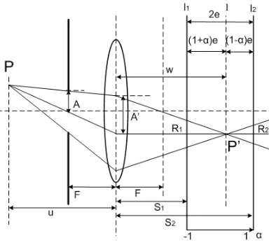
Fig. 1. The telecentric DfD system.
achieve high accuracy. However, the use of segmentation implies that the algorithm is only
suitable for objects on a flat surface.
Recent DfD methods also include those based on coded aperture (e.g., [12, 13]) which
customise the PSF by modifying the aperture shape, and most use a complex statistical
model which is computationally expensive. In [14] the image blurring effect is described
by oriented heat-flows diffusion, whose direction is determined from the local coherence
geometry, and the diffusion strength corresponds to the amount of blur. Using this method,
ridge-like artefacts on sharp edges are eliminated. In [15], an improvement on DfD is achieved
by manipulating exposure time and guided filtering. In [16], improvement is achieved by
minimising, via geometric optics regularisation, the information divergence between the
estimated and actual blurred images.
None of the above-mentioned methods achieves frequency independence without a
com-plex statistical model or training/testing based algorithm, i.e., the estimated depth is only
related to the blur size rather than the pattern of the blurred object. A solution is to
incor-porate a frequency parameter into the PSF as suggested in [17]. For most existing methods,
the depth is estimated from the ratio of two images with different degree of blur at a
par-ticular frequency. In contrast, the rational operator (RO) approach to DfD computes depth
using the normalised image ratio (NIR), or the M/P ratio which is a function of both depth
and frequency. The NIR is the ratio between the difference in the magnitude of two images
at all frequencies (M for minus) and the sum of the magnitude of them (P for plus). Due to
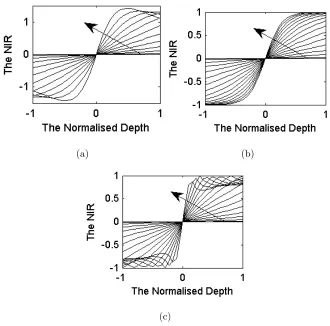
(a) (b)
(c)
Fig. 2. (a) The Pillbox NIR varies with the normalised depth. (b) Gaussian NIR with k=0.4578.
(c) Generalised Gaussian NIR with p=4 and k=0.5091. For each plot, the radial frequency of each
curve increases in the direction of the arrow. All the frequencies are shown as their ranges are
within [-1 1].
procedure has been proposed in [18] which also improves the depth estimation.
For convolved DfD, the telecentric optics described in [20] prevent an image magnification
effect that limits DfD. The telecentric RO-DfD system is illustrated in Fig. 1. The light rays
from an object pointP pass through the telecentric aperture of radius A, and then through
a circular part of radius A′ on the lens. The focused image of P is at l, a position between
the far-focused positionl1 and the near-focused image positionl2. The normalised depth α
is -1 at l1 and 1 at l2. The distance between l and l1 is (1 +α)e and that between l and
l2 is (1−α)e. A blurred circle of radius R1 and another of radius R2 are formed at l1 and
l2, respectively. The other parameters are denoted as follows: u is the distance between an
object point and the lens, ; F is the focal length;s1 is the distance between the lens andl1;
[image:5.612.140.470.77.403.2]Two images are captured: image i1 at l1, and image i2 at l2. When P is at far-focused
position, its focused image P′ is at l1. Similarly, when P is at near-focused position, its
focused image is at l2. Hence the working range of the RO-DfD system is from the
far-focused object position to the near-far-focused object position.
The NIR or the M/P ratio is defined as [20]
M
P (fr, α) =
H1(fr, α)−H2(fr, α) H1(fr, α) +H2(fr, α)
, (2)
whereH1 and H2 are respectively the PSFs of i1 andi2,α is the normalised depth which is
-1 when the focused image is on l1 and changes linearly from l1 to l2 so that it becomes 1
when it reaches l2, and fr is the radial frequency parameter in Hz. Using Eqn. (2) and the
Pillbox PSFs, curves representing the NIR changing with α are shown in Fig. 2(a), each of
which corresponds to a different discrete frequency. Each curve is modelled as a third order
polynomial of NIR with respect to the depth, as described by [20]
M
P (fr, α) =
Gp1(fr, α) Gm1(fr, α)
α+ Gp2(fr, α)
Gm1(fr, α)
α3, (3)
where the first order and third order coefficients are expressed as Gp1(fr, α)/Gm1(fr, α) and Gp2(fr, α)/Gm1(fr, α), respectively.
The corresponding spatial filters (the ROs) are then computed. During run-time, these
ROs are convolved with (i1−i2)(i1+i2) in a specific order as in [17] followed by a coefficient
smoothing procedure and a 7x7 post median filtering.
The advantages of RO based DfD in [17] include: (a) ability to produce a dense depth map
in real time with parallel hardware implementation; (b) the 3D reconstruction is invariant
to textures; and (c) the depth error can be as low as 1.18%. Therefore a RO based method
is feasible for real-time applications such as robotics and endoscopy. Its drawbacks are: (a)
using Pillbox PSF is only valid when the lens induced aberrations and diffraction are small
compared to the radius of the blur circle [19]; (b) a problematic filter design procedure used
in the Levenberg-Marquardt algorithm (see Section 2.B); (c) lack of careful consideration
on the NIR leads to the presence of some adverse frequency components. To address these
drawbacks, we propose two RO-based methods: the Gaussian rational operator (GRO) based
on the Gaussian PSF and the generalised Gaussian rational operator (GGRO) based on the
generalised Gaussian PSF.
The novelties of the proposed methods are: (1) the GROs address the situation when the
(RMSE); (2) a practical calibration method finds the linear relationship between the radius
of the blurred circle and the standard deviation of the Gaussian or the generalised Gaussian
PSF; (3) GGROs can be automatically configured to deal with the any levels of diffraction
and aberrations; (4) the ROs are designed with a new and simpler method; (5) the pre-filter
is redesigned to achieve better stability; and (6) an accurate and efficient DfD correction
method is presented in Section 3 to reduce the severe circular distortion encountered in any
DfD algorithm.
This paper is organised as follows. Section 2 presents the proposed GRO and GGRO
including the method for their calibration, a method for configuring GGRO, and the
pre-filter. Section 3 presents the DfD correction procedure. The experiments on real images and
discussion are presented in Section 4, and Section 5 concludes the paper.
2. The Proposed Rational Operators
The design of our proposed ROs involves three steps. The first step determines either the
Gaussian NIR or the Generalised Gaussian NIR. The second formulates the kernels of the
ROs from the corresponding NIR. The third formulates the pre-filter for both types of ROs.
2.A. The Gaussian NIR
When the aberrations and diffraction of the camera lens used in DfD are significant when
compared to the radius of the blurred circle, the Gaussian PSF is a better model than the
Pillbox PSF for modelling the image blur [19]. While the depth-related parameter of the
Pillbox model is the radius of the blurred circle, that of the Gaussian model is the standard
deviation (SD). The SD is related to the radius of the blurred circleRbyσ =kR[21], where
k is measured for the camera system used. Hence, unlike the Pillbox ROs that are generally
designed for every camera, the Gaussian ROs are designed for a specific camera system.
The 2D Gaussian PSF is [6]
h(x, y) = 1 2πσ2 exp
−(x−x)
2 + (y−y)2
2σ2
, (4)
where x−x and y−y are the distances between a point at (x, y) and the reference point
the Fourier transform of the PSF, i.e.,
H(u, v) =
Z Z 1
2πσ2 exp[C1] exp[−jux−jvy]dx dy, (5)
where C1 =−(x−x)2+(y−y)2
2σ2 . Rewriting the inner integral of Eqn. (5) as a quadratic function
of x, and using the quadratic exponential integration formula gives
H(u, v) =
Z
C2exp[C3 +C4]dy, (6)
where C2 = √1
2πσ2, C3 =
1 2
1
σx−juσ
2
, and C4 = −2σ12x2−
1
2σ2(y−y)2 −jvy. Similarly,
rewriting the integral as a quadratic function of y and using the quadratic exponential
integration formula gives
H(u, v) = exp
−1
2σ
2(u2+v2)
−j(xu+yv)
= exp
(−1 2σ
2(u2+v2)
exp[−j(xu+yv)]. (7)
In polar coordinates, the OTF is
H(r, θ) =rexp[−jθ], (8)
where the magnitude r = exp[−1 2σ
2(u2 +v2)], and the angle θ = xu+yv. Assuming the
OTF to be circular symmetric, it does not depend on angles and thus
H(u, v, σ) = exp
−1
2σ
2(u2+v2)
. (9)
σ is related to the blur circle radiusR by [21]
σ =kR, (10)
where k is a camera constant obtained by measurement. In this paper k is obtained as
follows:
1. Place a flat test pattern in front of the camera and perpendicular to the optical axis.
2. Focus the camera by computing its Fourier transform, where the image with the largest
high frequency magnitude is chosen as the sharpest (i.e., most focused). Denote the
position of the camera sensor asl1 (i.e., the far-focused sensor position) and the image
3. Move the sensor along the optical axis and away from l1 to the position of l2, such
that l2−l1 = 2e, where e is a constant as shown in Fig. 1. Capture the image as i2
(i.e., the near-focused image) at l2 (i.e., the near-focused position). Note that i1 is in
focus and i2 is blurred by a radius R= (1 +α)e/(2Fe).
4. Convolve image i1 with a Gaussian PSF of SD σt to generate image i′2t, i.e., i′2t = i1∗G(σt). The mean square error is ǫ(t) = mean(i2 −i′2t)2.
5. Repeat step (4) with a number of σt values. The estimated SD is given by σ1 =
arg minσtǫ(t).
6. Repeat steps 1-5 by makingi2 in focus and i1 blurred to get another approximation of
the SD σ2. The final estimated SD is σ = (σ1+σ2)/2, and k is σ/R. This is because
when the image is in focus oni1, the SD of the blurred circle oni2 is the same as that
oni1 when the image is in focus on i2.
Using trigonometric similarity in Fig. 1 gives
2R1
(1 +α)e =
2A′
w ,
where the effective f-number Fe isw/(2A′), so that
2R1
(1 +α)e =
1
Fe
⇒R1 = (1 +α)e 2Fe
. (11)
Substituting Eqn. (11) in Eqn. (10) and then in Eqn. (9) gives the far-focused OTF:
H1(u, v, α) = exp
"
−12
k(1 +α)e Fe
2
(u2+v2)
#
. (12)
The near-focused OTF is similarly obtained as
H2(u, v, α) = exp
"
−12
k(1−α)e Fe
2
(u2+v2)
#
. (13)
Note that the maximum radius of the blurred circle is optimally chosen to be 2.703 pixels
in [17, 18]. Thus according to Eqn. (11), the f-number (focal length divided by aperture
diameter) controls the sensor separation 2ewhich in turn controls the working range, where
noted from Eqn. (1) that a larger 2eresults in a larger difference in image positionwbetween
the far-focused and near-focused conditions. This leads to a larger difference between the
far and near object positions, i.e. the working range. This means a larger f-number results
in a larger working range and vice versa. However, a larger f-number will generate a higher
noise level in the data due to higher level of diffractions [6]. Notably, only the choices of
maximum radius and the f-number will change the experimental set-up, while the valuee is
determined by the radius and the f-number selected according to Eqn. (12).
An example Gaussian NIR graph is shown in Fig. 2(b), where k = 0.4578 as measured
for the camera system used to obtain the subsequently reported results. Unlike the
Pill-box NIR shown in Fig. 2(a), even the high-frequency curves of the Gaussian NIR increase
monotonically with depth. However, this does not mean they will not generate any adverse
effects. A discussion of this is presented in Section 2.D.
2.B. The Generalised Gaussian NIR
A 1-dimensional (1D) generalised Gaussian PSF, generated using a combination of the
Pill-box and Gaussian models with an adjustable parameter pis proposed in [22]. When p= 2,
it is equivalent to a Gaussian PSF, and when p → ∞ it is equivalent to the Pillbox PSF.
The 1-D generalised Gaussian PSF is [22]
h(x) = p
1−1p
2σΓ1p exp
−1p|x−x|
p
σp
, (14)
where Γ() is the Gamma function, σ is the SD such thatσ =kR,x is the spatial index and
x is the centre of the PSF. In this paper the value of p is obtained together with the value
k (using the method for determining k in Section 2.A) as follows:
1. Beginning with a very small value of p(e.g. p=1), find the mean square error ǫ(t) for
every attemptedσ(t). Store the minimum ofǫasE(p), and the correspondingk value
asK(p).
2. Repeat the previous step with a slightly larger p value (e.g., 0.1 larger), until the
minimum ofE(p) is identified. The estimated pvalue is given bypest = arg minpE(p),
DenotingC5 = 2σΓ1 p
p1p−1, Eqn. (14) becomes
h(x) = 1
C5
exp
−1p|x−x|
p
σp
, (15)
where C5 is used to keep the overall gain as 1. The equivalent 2D PSF is
h(x, y) = 1
C5 exp
−|x−x|
p+|y−y|p
pσp
. (16)
The OTF can be derived by the 2D Fourier transform of Eqn. (16), but no closed formed OTF
can be obtained. To address this problem, numerical methods such as Adaptive Simpson
Quadrature [23] can be used to calculate the OTF. The Fast Fourier Transform is a possible
alternative but it should be used with care. This is because when the SD is small, it fails
to produce accurate OTF values, whereas the Fourier transform by numerical integration
almost always give accurate results but is much slower to compute. Fig. 2(c) shows an
example of the NIR graph generated using p=4 and k=0.5091. As a result of the
Pillbox-Gaussian combination, each curve in the NIR graph has a smaller range than the Pillbox
NIR while the high-frequency curves do not increase monotonically with depth.
2.C. Design of the Rational Operators Kernels
Sections 2.A-2.B present the methods for finding the NIRs as given by Eqn. (3). The first
and third order coefficients can be found by performing a least squares fitting of the NIR.
The procedure used in [17] first setsGp1as the frequency response (FR) of a Log of Gaussian
(LOG) band-pass filter and then derives the other terms accordingly. The proposed method
adapts this procedure by using a different method to estimate the corresponding spatial
filters, i.e., the ROs.
In [17] and [18], the frequencies within [-0.5 0.5] Nyquist are divided into 32 discrete
portions to allow the polynomial coefficients to be found. Since the ROs operate in the spatial
domain, their FRs must be converted to the corresponding spatial filters. The elements of
the matrices (representing the filters) have to be real. Hence if they are determined by
inverse Fourier transform, the imaginary values violate this condition. In [17], the two
operators gm1 and gp2 are acquired by the Levenberg-Marquardt algorithm, where only one
cost function is used to find both gm1 and gp2. However, P(u, v;α) in [17] is assumed to
good approximation sinceP(u, v;α) is the FR of the sum of the two input images, and thus
cannot be a constant. Moreover, our experiments show that the weighting factor used in
their method significantly affects the optimisation result.
We solve this problem with a different cost function, which is the difference between the
left hand side and right hand side of Eqn. (2), i.e., to find the ROs, the FRs of which best
fit the NIR curves (this is also the final target of the ROs’ design in [17, 18]). Denoting
M
P (u, v, α) =
G′
p1(u, v) G′
m1(u, v)
α+ G
′
p2(u, v) G′
m1(u, v) α3
where (u, v) is the frequency index such that fr =
√
u2+v2, G′
p1, G′m1 and G′p2 are the
magnitudes of the FRs of the ROs gp1, gm1 and gp2 respectively, the cost function is given
by:
ǫ2 = X
u,v,α
M
P (u, v, α)·Fpre(u, v)−
M
P (u, v, α)
2
, (17)
where M
P is the NIR calculated using Eqn. (2) and Fpre is magnitude of the FR of the
pre-filter used to pre-filter the input images before DfD computation (see Section 2.D). Thus the
ROs are estimated as
[gp1, gm1, gp2] = arg min gp1,gm1,gp2
ǫ2. (18)
Therefore, all three ROs are estimated simultaneously, without approximating P(u, v;α).
In addition, the weight is set to be the same for every frequency index without the need
to compute it as a specific matrix as in [17]. This is because every frequency component
has even contribution to minimise the overall cost function of Eqn. (17). This results in the
right hand side of Eqn. (17) not having a denominator.
Eqn. (17) and (18) can be implemented with any non-linear optimisation algorithm such
as the Gauss-Newton algorithm, gradient descent algorithm or Levenberg-Marquardt
algo-rithm. A crucial step is the initialisation of ROs gm1 and gp2. As mentioned earlier, gp1 is
initialised as a LOG filter, then its FR Gp1 is calculated. Gm1 and Gp2 are then computed
with the estimated first and third order coefficients. The Parks-McClellan FIR filter design
algorithm and McClellan transformation are then used to find the initial guess for gm1 and gp2 [24, 25].
The procedure to initialise gm1 and gp2 is as follows: 1) Generate a 1D vector ftar by
sampling 6 values of the RO’s FR (Gm1 or Gp2) across 6 equally spaced frequency indices
the Parks-McClellan algorithm to find the 1D spatial filter f1d; 3) Use f1d as input to the
McClellan Transformation algorithm to get the corresponding 2D filter, which is the initial
guess for the RO (gm1 or gp2).
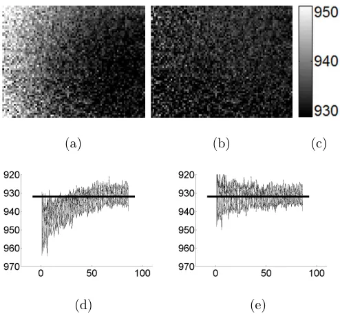
(a) (b) (c)
[image:13.612.181.428.137.365.2](d) (e)
Fig. 3. An example DfD correction problem. Grey-coded depth maps of a flat surface: (a) without
correction and (b) after correction. (c) The grey-bar of (a) and (b). Mesh plots: (d) the side view
of (a); and (e) the side view of (b), where the horizontal units are in pixel and the vertical units
are in mm. The horizontal lines in (d) and (e) represent the expected depth.
2.D. The pre-filter
The purpose of the pre-filter is to remove the frequency components which adversely affect
the accuracy and stability of the 3D reconstruction. To design the pre-filter appropriately,
these adverse frequency components are identified using a NIR graph, e.g., as is shown in
Fig. 2(b), as follows. For each frequency, if the variable represented by the vertical axis
in Fig. 2(b) (i.e., the NIR) is used as the input argument, and the output is the variable
represented by the horizontal axis.
Note that if the input varies even slightly, the resulting output depth will be highly
unstable. For example, for the second lowest frequency of 0.1963 Hz, represented by the
curve just next to the horizontal line, if the input varies within ±0.1, the output will vary
this problem since some parts of them are almost horizontal. Thus, a lack of consideration on
this problem can result in significant depth variation, requiring larger coefficient smoothing
and larger median filtering kernels (our experiments show that a 3x3 median filtering kernel
is typically enough to remove most high frequency noise, but it can be larger if the noise
power increases significantly) which slow down the processing.
The frequency components containing a large proportion of low-gradient or negative
gradient (corresponding to non-monotonicity) should thus be removed. This is achieved by
minimising the cost function
ǫ2 =X
u,v
F
pre(u, v)−Fpre′ (u, v) ζ(u, v)
2
, (19)
where Fpre is the target FR (to be determined later), Fpre′ is the FR of the estimated
pre-filter andζ is the weight matrix (to be determined later). In order to obtain a pre-filter that
effectively remove the components that introduce significant instability, which corresponds
to the NIR curves that contain parts with small or negative gradient, the corresponding
elements of Fpre need to be set small enough while maintaining Fpre to be smooth. In
addition, the weight matrix needs also be set in a way that the optimisation is focused on
obtaining small values for the adverse frequency components.
The optimal Fpre is obtained as follows: 1) Compute the gradients along each curve of
the NIRs at different depths; 2) Find the smallest gradient for each curve which corresponds
to a unique radial frequency fr; 3) Each element of Fpre is assigned by the smallest gradient
value (0 if negative) of corresponding curve with the same radial frequency fr =
√
u2+v2,
resulting in small values for the adverse components while enforcing smoothness of the filter;
4)Fpre is then divided by its maximum value to give a unity gain filter; 5)ζ(u, v) is set to be
Fpre incremented by a small value (e.g., 0.05) so that it does not contain zero, resulting in
the optimisation focused on the adverse components. The optimisation can be implemented
by one of the non-linear optimisation methods, initialised with the same method as the ROs
as presented in Section 2.C.
3. DfD Correction Method
During numerous experiments using three different lenses (a professional 50 mm lens, a 35
observed using all the DfD algorithms mentioned in Section 1. Such a problem is illustrated
in Fig. 3. Here a hill-like result is generated from a flat plane that is perpendicular to the
optical axis. The hill is more or less circularly symmetric which is similar to the surface
of a common lens. Also its centre deviates from the centre of the map due to the focus
adjustment during the experiment. An analysis of the experiment reveals the following
concern. When an image is defocused by moving the sensor, it cannot be defocused evenly
across the image, where some parts are more blurred than the others (the shape of the
defocused pattern is similar to the distorted depth map in Fig. 3(a), where the varying grey
levels denote the uneven surface). In addition, the small f-number used results in a narrow
depth of field, making the problem easily observed. In other words, the distorted blur field
leads to a distorted depth map. Note that both results are generated with the same scale
using Watanabe’s [17] DfD method. The expected depth map should be flat with a value of
933 mm.
Generally, it is possible to correct either the input images or the output depth map.
The former is considered not practical due to the complex measurement involved, so the
proposed method is based on correcting the output depth maps. An immediate thought is
to subtract any depth map by a calibration pattern (i.e., the depth map generated for the
far-focused object position) and then minus the expected depth of that pattern (the depth
offset). However, our experiments show that the appropriate calibration pattern is depth
dependent. Thus, a closed-form solution is needed to find the correction factor for each
element of the pattern.
The offset ∆ at the location defined by the Cartesian coordinates (x, y) is modelled
as a third order polynomial of the coordinates x and y and the corresponding raw depth
uraw(x, y), i.e.,
∆(x, y) =c1(1) +
4
X
i=2
c1(i)xi−1+ 7
X
i=5
c1(i)yi−4+ 10
X
i=8
c1(i)(uraw(x, y))i−7. (20)
Samples of ∆ and uraw are obtained by capturing a pair of DfD images of a test flat
surface at a location within the working range, e.g., ∆ is -1, when the surface is at the
far-focused object point, and uraw is thus the corresponding computed depth map. The
given by
uc(x, y) = c2(1) + 4
X
i=2
c2(i)xi−1+ 7
X
i=5
c2(i)yi−4+ 10
X
i=8
c2(i)(∆(x, y))i−7, (21)
whereuc(x, y) is equivalent to uraw(x, y), and ∆(x, y) is found by the previous step and the
coefficient vector c2 is similarly computed with a least square fit. Finally, to correct any
depth result at a specific location (x, y), the following procedure is required:
1. The location coordinate (x, y) and the uncorrected result uraw are substituted into
Eqn. (20) to get the offset ∆(x, y).
2. The location coordinate (x, y) anduc(x, y) are substituted into Eqn. (21) to compute
the correction factoruc(x, y).
3. The corrected depth is thus estimated by ucorrected(x, y) = uraw(x, y)− uc(x, y) +
∆(x, y).
An example of the corrected depth map is shown in Fig. 3(b) and (e), where the working
range is within [886.8 933] mm away from the lens. To show that the correction method
works with any RO-DfD, the depth results are generated using Watanabe’s ROs [17]. While
the local noise level is not visibly magnified, the general shape of the hill has been restored
to be flat. A typical correction of a depth map only accounts for 4-8% of the total RO-DfD
computational time, hence it is suitable for real-time applications.
4. Experiment
Since the proposed RO-DfD methods are based on different PSFs than those used in [17]
and [18], experiments with simulated images are not of any use because they are generated
with a specific PSF. Thus we only discuss the depth results using real images. In addition,
since the ROs in the Raj’s method [18] produce better results than the ROs in [17], the
comparison is made between the state-of-the-art Raj’s method and the proposed method.
A professional 50 mm lens is used with a telecentric aperture whose diameter is 12.8 mm.
The f-number Fe is thus obtained by dividing the focal length F = 50 mm by the aperture
diameter 2A= 12.8 mm, which is 3.9063. The side-length of each CCD sensor element is 7.4
circle is 2.703×7.4−3 = 0.0200 mm The far-focused object position u
1 is set 933 mm away
from the lens.
The working range is computed as follows:
1. When radius of the blurred circle on l1 is 0 the scene is far-focused such that s1 =w,
substituting u = u1 = 933 mm and F = 50 mm into Eqn. (1) gives the far-focused
sensor-lens separation s1 =w= 52.8313 mm.
2. When radii of the blurred circles onl1andl2are respectively of 0.02000 (the maximum)
mm and 0 (the minimum), substituting R1 = 0.0200 mm, α = 1 (this is true when R1 reaches its maximum) and Fe = 3.9063 into Eqn. (11) gives the sensor separation
2e= 0.1563 mm, such that the near focused sensor-lens separation is s2 = s1+ 2e =
52.9876 mm.
3. When radius of the blurred circle onl2 is 0 as in step 2, substitutingw=s2 = 52.9876
mm and F = 50 mm into Eqn. (1) gives the near-focused object position u2 = u =
886.8 mm. Thus the working range is [886.8 933] mm away from the camera.
The input image resolution is 640×480. The proposed RO-DfD method is implemented
on a computer with an Intel Pentium Dual-Core 2.16 GHz processor. A flat surface covered
with sandpaper is used as the test pattern for evaluation. It is set perpendicular to the
optical axis and shifted from the far-focused object position to the near-focused position,
with successive locations separated equally by 46.18/23 mm. 24 pairs of images are thus
captured and 24 depth maps computed.
A 7×7 window is used for coefficient smoothing. For comparison with Raj’s method, the
Root Mean Square Error (RMSE) is measured between the estimated depth map and the
ideal flat depth map for each pair of inputs. A set of 24 measurements is obtained for each
one of Raj’s method, GRO and GGRO. Here the k value for GRO is estimated as 0.4578
using the method presented in Section 2.A; p and k for GGRO are respectively estimated
as 1.8 and 0.4802 using the method presented in Section 2.B.
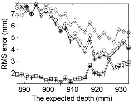
Fig. 4 shows the comparisons of RMSE between Raj’s ROs [18] and the ROs (i.e., the
Gaussian based and the Generalised Gaussian based) of the proposed method.
Note that the proposed DfD correction method only deals with the general shape of
Fig. 4. Comparison of RMSE of
Raj’s and the proposed methods. Key: ♦- Raj; - GRO uncorrected;∗ - GGRO uncorrected;
- GRO corrected; and + - GGRO corrected.
noise level as illustrated in Fig. 3. In addition, experiments show that the RMSE before
correction is dominated by the general shape and depends on the local noise level after
correction. Furthermore, the general shape distortion is worse for the smaller depths than
the larger ones, while the local noise level is worse for the larger depths than the smaller
ones. Thus, for the uncorrected results shown in Fig. 4 the RMSE is higher for the smaller
depths than the larger depths, while the RMSE after correction is higher for larger depths
than smaller depths.
Despite all these general RO-DfD problems, the results before correction of the proposed
ROs are more accurate than using Raj’s ROs for depths larger than 890.8 mm while GGROs
produce the least overall RMSE. Moreover, for the results after correction, the proposed
(a) (b) (c) (d)
(e) (f) (g) (h)
(i) (j) (k) (l)
[image:19.612.90.527.68.586.2](m) (n) (o) (p)
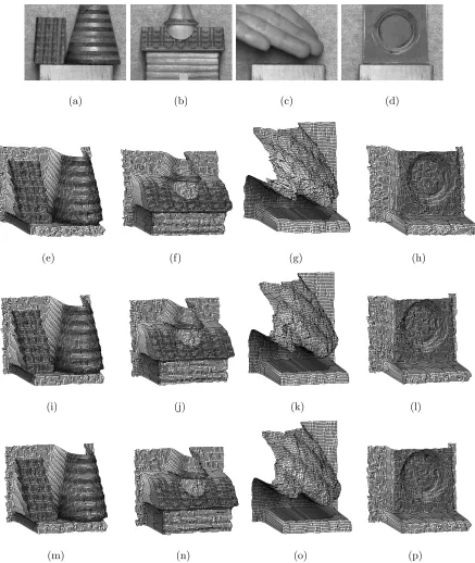
Fig. 5. Wireframe plots of the results using Raj’s and the proposed methods with the test objects.
Row 1 - the test scenes. Mesh plots of 3D scene reconstructions using: row 2 - Raj’s method; row 3
- GRO; and row 4 - GGRO. Note that the results in column 3 are generated using 5x5 post median
Fig. 5 show the four real test scenes comprising different shaped objects for evaluating the
performance of the proposed method qualitatively. Note that our experiments show that 3x3
post median filtering (PMF) is typically sufficient to remove most noise while preserving the
depth discontinuity for scenes that are not reflective and having visible textures. However
the results in the third column are generated using 5x5 PMF instead of 3x3 PMF. This is
because the associated scene of the fingers is considerably more reflective than the others and
does not have sufficient textures to enable DfD to work with blurring. For a scene with no
or little texture, there is little different in blur with the two captured images. When the
pre-filter fails to remove some adverse frequency components, e.g., low frequencies corresponding
to little texture, high noise level is perceived (see Section 2.D). For the staircase and cone
scene in the first column, there is less noise in the reconstructed surface and the circular
distortion is eliminated. The wooden temple results in the second column test the algorithms
with complex objects that do not span the full working range, where the expected range of
the temple is significantly lower than than the working range. Similar results are obtained.
The third column shows the advantage of the smoothing nature of the GRO, which removes
much of the low-frequency components (due to the reflective hand surface) while preserving
the depth discontinuity. The object with a conical depression shown in the last column is
used to demonstrate the ability of the DfD correction method to cope with multiple depths.
[image:20.612.169.435.523.678.2]Here not only is the background corrected, but the foreground objects are also corrected.
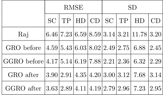
Table 1. The mean RMSE and the mean SD of all the flat surfaces in the reconstruction results of
the test scenes in Fig. 5, before and after correction. All units are in mm.
RMSE SD
SC TP HD CD SC TP HD CD
Raj 6.46 7.23 6.59 8.59 3.14 3.21 11.78 3.20
GRO before 4.59 5.43 6.03 8.02 2.49 2.75 6.88 2.45
GGRO before 4.17 5.14 6.19 7.88 2.21 2.36 6.32 2.29
GRO after 3.90 2.91 4.35 4.20 3.00 3.12 7.68 3.14
GGRO after 3.63 2.89 4.11 4.19 2.79 2.96 7.23 2.95
Table 1 shows the numerical comparisons based on the four sets of results. In these tables,
and Conical depression that are shown in Fig. 5(a)-(d), respectively.
Column 2-5 in Table 1 shows the comparison of the RMSE between Raj’s results and
the proposed ones, generated from the four sets of results. The RMSE for each test scene
is measured as follows. For each flat surface that is perpendicular to the optical axis, the
RMSE is calculated between the estimated depth and the actual depth which is measured
with a vernier calliper. The average of these RMSEs is used as the RMSE for the scene. The
table shows that both GRO and GGRO produce smaller RMSE than Raj’s method, while
GGRO produces the smallest RMSE. Moreover, the correction method manages to reduce
the RMSE significantly.
Column 6-9 in Table 1 compares the noise levels between Raj’s results and those of the
proposed methods, which are measured by the average SD of the flat surfaces of the four sets
of results. For example, for the scene in the first column of Fig. 5, the SD is evaluated for
each step surface of the staircase, the surface of the wooden chunk at the bottom, and the
background. The average of these SDs is used to indicate the noise level of the depth result.
The table shows that both GRO and GGRO produce less noise than Raj’s method, while
GGRO generates the least noise. In addition, the correction method has little influence on
the noise level.
In terms of the computing time, the proposed depth estimation and depth correction only
take typically 0.35 second. If a parallel hardware implementation is used, a real-time DfD
processing is also achievable. Therefore the proposed DfD method can be very useful for
robotic and medical applications.
5. Conclusion
Lens aberrations and diffraction are two undesirable and unavoidable imperfection in image
acquisition where 3D object reconstruction techniques including DfD suffers. The former
occurs when sub-quality lenses are used and the latter occurs when small aperture is used
or the image centre is misaligned with the optical axis [26]. This paper presents two novel
RO-DfD methods, one using Gaussian PSF and another using Generalised Gaussian PSF.
The GROs cope well in situations where the lens aberrations and diffraction are significant
compared to the blur radius. The GGROs can cope with any levels of aberrations and
the measurement of depth as well as its monotonicity. Moreover, the ROs are designed to
speed up the filters generation process.
The paper also presents a practical DfD correction method that addresses the circular lens
distortion and misalignment between the image centre and the optical axis. Experiments
on real images with both quantitative and qualitative results show that the GROs and
the GGROs together with the proposed correction algorithm respectively produce more
accurate results than the state-of-the-art Raj’s ROs. Furthermore, the proposed methods
are fast with the effective and efficient correction stage eliminating the hill-like depth map
distortion generated by existing DfD methods.
Our method works well because: 1) GROs use Gaussian model that is more suitable
than the Pillbox model for defocusing that is dominated by aberrations and diffraction; 2)
GGROs use generalised Gaussian model that generalises the RO-DfD method to deal with
any levels of aberrations/diffraction; 3) Input frequency components are analysed using the
NIR and removed with a pre-filter; 4) The ROs are designed with a simpler method achieving
comparable accuracy than [17, 18]; 5) A simple DfD correction procedure is devised to
eliminate the strong circular distortion originated from image acquisition.
Although our method works effectively, the general shape of the NIR cannot be
repro-duced without error and the adverse frequency components cannot be removed completely
due to the small-sized broad-band ROs. We will investigate as a future work the use of coded
aperture to produce a PSF suitable for small ROs. Moreover, the current implementation
of the proposed methods requires the sensor to be moved from one position to another with
typical precision of 5 µm. To increase the precision, we will investigate the use of a step
motor or a batch of piezoelectric-electric materials to control the movement. If the size of
the camera system is not an issue, two sensors and a half mirror could be used to remove
the need to move the sensors.
6. Acknowledgement
References
[1] R. Minhas, A. A. Mohammed and Q. M. J. Wu, “Shape from focus using fast discrete curvelet
transform,” Pattern Recognition 44, 839-853 (2011).
[2] I. Lee, M. T. Mahmood, S. Shim and T. Choi, “Optimizing image focus for 3D shape recovery
through genetic algorithm,” Multimedian Tools and Applications, DOI:
10.1007/s11042-013-1433-9.
[3] M. Born and E. Wolf,Principles of Optics (Pergamon, 1965).
[4] S. Chaudhuri and A. N. Rajagopalan,Depth From Defocus: a Real Aperture Imaging Approach
(Springer, 1998).
[5] A. P. Pentland, “A new sense for depth of field,” IEEE Transactions on Pattern Analysis and
Machine Intelligence PAMI-9, 523-531 (1987).
[6] M. Subbarao, “Parallel depth recovery by changing camera parameters,” in Proceedings of
IEEE ICCV (IEEE, 1988), pp. 149-155.
[7] J. Ens and P. Lawrence, “An investigation of methods for determining depth from focus,”
IEEE Transactions on Pattern Analysis and Machine Intelligence 15, 97-108 (1987).
[8] Y. Xiong and S. A. Shafer, “Moment and hypergeometric filters for high precision computation
of focus, stereo and optical flow,” International Journal of Computer Vision 22, 25-59 (1997).
[9] A. N. Rajagopalan and S. Chaudhuri, “An MRF model-based approach to simultaneous
recov-ery of depth and restoration from defocused images,” IEEE Transactions on Pattern Analysis
and Machine Intelligence 21, 577-589 (1999).
[10] P. Favaro and S. Soatto, “Learning shape from defocus,” in Proceedings of 7th European
Conference on Computer Vision (Springer, 2002) pp. 735-745.
[11] L. Ma and R. C. Staunton, “Integration of multiresolution image segmentation and neural
networks for object depth recovery,” Pattern Recognition 38, 985-996 (2005).
[12] A. Levin, R. Fergus, F. Durand, “Image and depth from a conventional camera with a coded
aperture,” ACM Transactions on Graphics (TOG) 26, 70 (2007).
[13] C. Zhou, S. Lin and S. Nayar, “Coded aperture pairs for depth from defocus and defocus
deblurring,” Int. J. Comput. Vis 93, 53-72 (2011).
[14] L. Hong, J. Yu and C. Hong, “Depth estimation from defocus images based on oriented
pp. 212-215.
[15] H. Wang, F. Cao, S. Fang, et al., “Effective improvement for depth estimated based on defocus
images,” Journal of Computers 8, 888-895 (2013).
[16] Q. F. Wu, K. Q. Wang, and W. M. Zuo, “Depth from defocus using geometric optics
regular-ization,” Advanced Materials Research 709, 511-514 (2013).
[17] M. Watanabe and S. K. Nayar, “Rational filters for passive depth from defocus,” International
Journal of Computer Vision 27, 203-225 (1998).
[18] A. N. J. Raj and R. C. Staunton, “Rational filter design for depth from defocus,” Pattern
Recognition 45, 198-207 (2012).
[19] M. Born and E. Wolf,Principles of Optics: Electromagnetic Theory of Propagation,
Interfer-ence and Diffraction of Light (CUP Archive, 1999).
[20] M. Watanabe and S. K. Nayar, “Telecentric optics for focus analysis,” IEEE Transactions on
Pattern Analysis and Machine Intelligence 19, 1360-1365 (1997).
[21] M. Subbarao and G. Surya, “Depth from defocus: a spatial domain approach,” International
Journal of Computer Vision 13, 271-294 (1994).
[22] C. D. Claxton and R. C. Staunton, “Measurement of the point-spread function of a noisy
imaging system,” JOSA A 25, 159-170 (2008).
[23] W. Gander and W. Gautschi, “Adaptive quadrature–revisited,” BIT Numerical Mathematics
40, 84-101 (2000).
[24] IEEE Acoustics, Speech, and Signal Processing Society. Digital Signal Processing Committee,
Programs for Digital Signal Processing (IEEE, 1979).
[25] J. S. Lim,Two-Dimensional Signal and Image Processing (Prentice Hall, 1990).
[26] S. F. Ray, Applied Photographic Optics: Imaging Systems for Photography, Film and Video