warwick.ac.uk/lib-publications
Original citation:
Kim, Gi Hyun, Li, Haitao and Zhang, Weina. (2016) CDS-bond basis and bond return predictability. Journal of Empirical Finance, 38 . pp. 307-337.
Permanent WRAP URL:
http://wrap.warwick.ac.uk/81653 Copyright and reuse:
The Warwick Research Archive Portal (WRAP) makes this work by researchers of the University of Warwick available open access under the following conditions. Copyright © and all moral rights to the version of the paper presented here belong to the individual author(s) and/or other copyright owners. To the extent reasonable and practicable the material made available in WRAP has been checked for eligibility before being made available.
Copies of full items can be used for personal research or study, educational, or not-for-profit purposes without prior permission or charge. Provided that the authors, title and full bibliographic details are credited, a hyperlink and/or URL is given for the original metadata page and the content is not changed in any way.
Publisher’s statement:
© 2016, Elsevier. Licensed under the Creative Commons Attribution-NonCommercial-NoDerivatives 4.0 International http://creativecommons.org/licenses/by-nc-nd/4.0/
A note on versions:
The version presented here may differ from the published version or, version of record, if you wish to cite this item you are advised to consult the publisher’s version. Please see the ‘permanent WRAP url’ above for details on accessing the published version and note that access may require a subscription.
1
CDS-Bond Basis and Bond Return Predictability
Gi H. Kim Haitao Li Weina Zhang1
July 2016
Abstract
We examine the predictive power of the CDS-bond basis for future corporate bond returns. We
find that residual basis, the part of the CDS-bond basis that cannot be explained by a wide range
of market frictions such as counterparty risk, funding risk, and liquidity risk, strongly negatively predicts excess returns. Controlling for systematic risk factors, including credit risk and liquidity risk, we find that a bond portfolio formed on the residual basis generates a significant abnormal bond return of 1.79% at the 20-day horizon. The abnormal returns due to the residual basis reflect mispricing rather than missing systematic risk factors. These results are robust to different horizons and sample periods and to the various characteristics of bonds. Overall, our results imply a beneficial role of CDS in the bond market as the existence of mispricing between CDS and bonds results in a subsequent price convergence in bonds.
JEL Classification: G10, G12
Keywords: Credit default swaps, CDS-bond basis, basis arbitrage, corporate bonds, financial crisis, limits of arbitrage, return predictability, price convergence
1 Kim is from the Finance Group, Warwick Business School, University of Warwick. His email is at [email protected]. Li is from Cheung Kong Graduate School of Business, Beijing 100738. His email is at
[email protected]. Zhang is from Department of Finance, NUS Business School, National University of Singapore. Her email is at [email protected].
2
1. Introduction
The market for credit default swaps (CDS) has seen tremendous growth in recent years. According to the Bank for International Settlements (BIS, 2010), the notional value of outstanding credit derivatives at the end of 2007 was $58 trillion, more than six times that of the corporate bond market. As a result, CDS have fundamentally changed market practices in the investment, trading, and management of credit risks. As CDS are essentially an insurance contract against the default of a company’s bonds, the CDS and corporate bond markets tend to move in tandem, closely interacting with each other.
The CDS basis (“the basis” hereafter), the deviation between CDS and bonds spreads, is one of the well-known no-arbitrage relations. In theory, the basis should be close to zero, ignoring some technical issues and market frictions. The violation of this relation, if any, may represent the relative mispricing between corporate bonds and CDS. Much interest has been shown, by both academics and practitioners, in understanding the basis, especially after the recent financial crisis, when an extremely negative basis was observed. Most of the existing studies on the analysis of the basis are centered on the causes of the non-zero basis (e.g., Bai and Collin-Dufresne, 2014; Fontana, 2011; Longstaff, Mithal, and Neis, 2005). No prior study, however, has addressed the implications of the basis for future price movements in related markets. Our study fills this void by investigating the predictive power of the basis for future returns in the corporate bond and CDS markets.
3
being corrected instantly (Duffie, 2010). A recent study by Bai and Collin-Dufresne (2014) documents that 34% of the CDS-bond basis can be explained by risks or market frictions (e.g., illiquidity). If a large portion of the basis cannot be explained by known factors, the remaining part of the non-explainable basis can potentially reflect temporary “mispricing,” which may converge at zero in the future. Therefore, the non-zero basis may predict a price convergence in future periods of the corporate bond and CDS markets. Such predictability is expected to be stronger for the less efficient bond market than for the more efficient CDS market. Using a refined measure of the non-zero basis, we aim to quantify the predictive power of the mispricing between bonds and CDS for their future returns.
To filter out the impact of market frictions and risks involved in a typical basis arbitrage, we separate the observed basis into two parts based on the empirical explanatory model of basis by
Bai and Collin-Dufresne (2014): (1) predicted basis, which captures the equilibrium non-zero
level of the basis due to market frictions and risks (such as counterparty, funding, and liquidity
risk); and (2) residual basis, which captures the unexplained part of the basis that may reflect
mispricing between bonds and CDS. Although the residual basis may not be fully devoid of market frictions or risk factors that are not specified in the empirical model, it is expected to be less noisy in capturing mispricing after removing the well-known risks and measurable market frictions.2
We first document that the residual basis strongly predicts future returns for corporate bonds. We find that a one standard deviation increase in the residual basis predicts a negative future
2 Anecdotal evidence suggests that basis arbitrageurs will start trading only when the basis crosses a certain
4
excess bond return of –4.8% on an annual basis at a minimum, suggesting that currently overpriced (underpriced) corporate bonds relative to CDS experience a subsequent price decline (increase). The price correction of corporate bonds occurs over various time horizons (e.g., 20 days, 40 days, and 60 days). The predictive power of the residual basis is still robust after
controlling for bond illiquidity,3 information spillover from the CDS market, and price
momentum and reversals. However, the predicted basis has a much lower predictive power for future bond returns.
A typical basis arbitrage also involves CDS since arbitrageurs tend to hedge their bond positions with CDS. When the basis is negative (positive), one can long (short) the underlying corporate bond and buy (sell) CDS to bet on the narrowing of the basis. The arbitrage force may lead to an adjustment in subsequent CDS prices. Our empirical results confirm this intuition by showing that the residual basis has strong predictive power for the change in CDS spreads as well. A one standard deviation increase in the residual basis predicts a rate of change in CDS spreads of –11.9% on an annual basis at a minimum, suggesting that the corresponding CDS experience a subsequent spread decrease. However, the predicted basis does not predict CDS price movements at all.
Even though the residual basis has strong predictive power for both markets, the statistical significance of its predictability is much stronger for bond markets than for CDS markets. The t-statistics for the coefficients on the residual basis in our predictive regression models are about two times bigger for bond markets than for CDS markets, regardless of model specifications.
3 See, for example, Longstaff, Mithal, and Neis (2005); Chen, Lesmond, and Wei (2007); Goldstein, Hotchkiss, and
5
This result is also consistent with the literature documenting that mispricing is observed more often in bond markets than in CDS markets because CDS markets are more efficient in pricing credit risk (e.g., Acharya and Johnson, 2008; Blanco, Brennan, and Marsh, 2004).
We perform several robustness tests to ensure that the strong predictability is consistent with the mispricing and subsequent price convergence interpretation. It is well known that investment-grade (IG) and high-yield (HY) bonds are different in many dimensions, such as investors’ clientele and liquidity (e.g., Da and Gao, 2010; Acharya, Amihud, and Bharath, 2013). Therefore we analyze each type of bond separately. Our results show that the price corrections occur for both types of bonds across different time horizons (20 days, 40 days, and 60 days), but the result is weaker for the speculative-grade CDS over longer horizons ( 40 days or 60 days). This result is consistent with the anecdotal evidence that the basis arbitrage is risky and that basis arbitrageurs opt for safer investment opportunities, such as investment-grade credit instruments and shorter horizons (e.g., Deutsche Bank, 2009).
Given the disruption of the corporate bond and CDS markets during the financial crisis,4 we
also investigate whether price corrections were disrupted during the crisis. Our results show that the predictability of the residual basis for bond price correction was still robust during the crisis. Interestingly, the predictability for CDS spread movement was not statistically significant during the crisis. These results indicate that basis arbitrage plays a reduced role in stabilizing the CDS market during a crisis, consistent with the literature that the limits of arbitrage have been hit by investors (e.g., Duffie, 2010; Mitchell and Pulvino, 2012).
4 For example, see Fontana (2011); Trapp (2010); Dick-Nielsen, Feldhütter, and Lando (2012); Friewald,
6
Given the strong predictive power of the residual basis for future bond returns, it is natural to verify whether we could implement a profitable convergence trade in bond markets based on the residual basis as a trading signal. Indeed, we find that a strategy of buying low-residual corporate
bonds and selling high-residual corporate bonds earns a statistically significant high abnormal
return of 1.79% over a 20-day horizon. The return is even higher for longer horizons in which we have 2.40% for a 40-day, and 2.68% for a 60-day horizon. This result is robust after controlling for well-known systematic risk factors for corporate bonds, including default and liquidity risk factors as well as various bond characteristics such as credit ratings, maturity, age, coupon, and issue size. Even after taking into account the fact that corporate bonds may incur high transaction costs, these returns are still sizeable (especially for an institutional investor).5 However, a similar trading strategy based on the predicted basis generates much less economically and statistically significant abnormal returns. Specifically, the abnormal return from predicted basis arbitrage strategy is 0.67% for a 20-day horizon, which is less than a half the return from the residual basis. These results suggest that the residual basis can serve as a much better trading signal for arbitrageurs who wish to exploit the mispricing between the bond and CDS markets.
The final test we perform is to confirm that the source of the high abnormal bond returns is
due to “pure” mispricing rather than to unknown or missing risk factors. Following the standard
approach in the literature (e.g., Fama and French, 1993; Daniel and Titman, 1997; Gebhardt, Hvidkjaer, and Swaminathan, 2005), we compare the explanatory power of the cross-section of bond returns of the residual basis itself with a factor-mimicking portfolio, the Low-minus-High (LMH) factor, which is based on the residual basis. Our results show that when the residual basis
5 Edwards, Harris, and Piwowar (2007) show that the average round-trip cost for a representative retail order size of
7
itself is included in the return regression, the LMH factor does not explain the bond returns, while the residual basis is significantly related to the bond returns. This finding suggests that the residual basis represents temporary mispricing in corporate bonds rather than unknown risk factors.
Our study makes three distinct contributions to the existing literature. First, our results contribute to the rapidly growing literature on the CDS-bond basis. The non-zero CDS-bond basis is still a puzzle that is yet to be understood in full. For the aggregate level of the basis, Fontana (2011) studies the basis during 2007/09 financial crisis for investment-grade U.S. firms and shows that the basis is correlated with a few factors, including the Libor-OIS spread. Fontana and Scheicher (2010) examine the sovereign basis for ten European countries to understand the determinants of the basis. For the cross-section of the basis, Bai and Collin-Dufresne (2014) utilize a risk-return analysis on the basis and suggest potential explanations for the basis, such as market frictions and bond characteristics. Nevertheless, they are able to explain only 34% of the basis variations. There are many more unknown “limits to arbitrage” reasons that contribute to the non-zero basis. Our findings shed new light on the source of the non-zero basis by showing that a residual basis represents a better measure of mispricing.
8
document the price convergence between derivatives and underlying cash securities in the credit markets.
Last, our study also contributes to the recent debate over whether CDS improve the overall efficiency and quality of other related markets. Boehmer, Chava, and Tookes (2013) find that CDS generally have a negative impact on equity market quality measured in terms of stock liquidity and stock price efficiency. Das, Kalimipalli, and Nayak (2014) also argue that CDS are largely detrimental to the corporate bond market, which has become less efficient and has not
experienced a reduction in pricing errors or an improvement in liquidity.6 Our finding that price
adjustments are stronger in the corporate bond market than in the CDS market, however, suggests that the presence of CDS may improve the pricing efficiency of the corporate bond market.
The rest of the paper is organized as follows. Section 2 discusses the construction of the residual basis. Section 3 presents our main result that the residual basis predicts price convergence between CDS and corporate bonds. Section 4 shows that the return predictability by the residual basis is not due to missing risk factors but captures mispricing in corporate bonds. Section 5 presents several robustness tests and section 6 concludes.
2. Residual Basis: A Refined Measure of Mispricing
In this section, we explain how our basis measure is constructed, from which we describe how to develop a refined measure of the mispricing between CDS and corporate bonds, devoid of
6 Our paper also differs from Kim, Li, and Zhang (2013), who study CDS-bond basis arbitrage. They interpret the
9
various market frictions and risks that may prevent arbitrageurs from exploiting price discrepancies.
2.1. Methodology
The basis for a given firm i at time t for a given maturity τ is defined as
, , , , , , ,
i t i t i t
Basis CDS Z (1)
where CDSi,t,τ is the CDS spread of firm i at time t with maturity τ, and Zi,t,τ is the Z-spread. The
Z-spread, which is widely used in industry to define the basis (e.g., Choudhry, 2006), represents a parallel shift of the credit curve such that the present value of future cash flows equals the current price. For a 5-year plain vanilla bond with an annual coupon, we obtain the Z-spread by solving the following equation:
2 3 4 5
1 2 3 4 5
1 ,
(1 c ) (1 c ) (1 c ) (1 c ) (1 c )
P
s Z s Z s Z s Z s Z
(2)
where P is the current price of the bond with a face value of 1, c is the coupon rate, si is the
zero-coupon yield to maturity based on the swap rate curve for a maturity of i year(s) (where i = 1,
2,…, 5). Then we match the Z-spread with the CDS spread at the same maturity. If we do not have an exact match for maturity, we linearly interpolate the CDS curve to obtain a CDS spread that has the same maturity as the bond.
10
payments,7 or (ii) risks encountered in a basis arbitrage (such as counterparty, funding, and liquidity risks).
Based on an empirical model developed by Bai and Collin-Dufresne (2014),8 which is
described in Appendix A.1, we separate the basis into two parts: “predicted basis,” which represents the equilibrium non-zero level of the basis, and “residual basis,” which cannot be explained by known risk factors and on average has a value of zero. To the extent that the predicted basis captures risks and market frictions encountered in a basis arbitrage, our residual basis measure should be a less noisy measure than the overall basis for capturing the pure mispricing between bonds and CDS.
2.2. CDS and Bond Data
The CDS data used in this study are on standardized ISDA contracts for physical settlement. We obtain the CDS data from Markit, which aggregates quotes from major CDS dealers. We focus on U.S. dollar-denominated CDS contracts that are senior unsecured with the “Modified Restructuring” clauses from 2001 through 2008. The daily CDS spreads are quoted in basis points (bps) per year for a notional amount of $10 million. While previous studies have mainly focused on CDS contracts at a five-year maturity, we use the complete curve of CDS spreads for 6-month, 1-, 2-, 3-, 5-, 7-, 10-, 15-, 20-, and 30-year maturities to exact-match the maturities of corporate bonds. The bond data for the years 2001 through 2008 are obtained from three
7 It might be difficult to find a CDS with exactly the same maturity as the cash bond. In a default event, when the
accrued interest is paid upon default in CDS, it may not be paid for the defaulted bond. Interest for CDS is paid quarterly, whereas it is paid semi-annually for most cash bonds. The cheapest-to-deliver option embedded in a CDS contract can be extremely valuable in some default events, which could lead to discrepancies between CDS and bond spreads.
8 We are aware that Nashikkar, Subrahmanyam, and Mahanti (2011) have proposed an alternative empirical
11
different sources. The price information is from TRACE and NAIC, bond transaction databases that have been widely used in recent literature. The bond transaction data are further merged with the Fixed Investment Securities Database (FISD) to obtain bond characteristic information, such as issue dates, maturity dates, issue amount, and rating information. To compute the basis, we focus on senior-unsecured fixed-rate straight bonds with semi-annual coupon payments, and delete bonds without credit ratings from any of the three rating agencies (Standard & Poor's, Moody's, and Fitch). We further remove bonds with embedded options (callable, puttable, or convertible bonds), floating coupons, and less than one year to maturity.
TRACE was officially launched in 2002 by the Financial Industry Regulatory Authority (FINRA), which replaced NASD, to disseminate secondary over-the-counter (OTC) corporate bond transactions by its members. TRACE has gradually increased its coverage of the bond market over time. By July 1, 2005, FINRA required all its members to report their trades within 15 minutes of the transaction. Nowadays, TRACE covers all trades in the secondary over-the-counter market for corporate bonds and accounts for more than 99% of the total secondary trading volume in corporate bonds. The only trades not covered by TRACE are trades on the NYSE, which are mainly small retail trades. The information contained in TRACE includes transaction dates and transaction price (clean price or price with commissions). In this study we exclude transactions whose prices are mixed with commissions.
12
half of 2002 (Schultz , 2001; Campbell and Taksler, 2003). A recent study by Lin, Wang, and Wu (2011) also uses the combined dataset of NAIC and TRACE to study the liquidity risk in the corporate bond market. NAIC is an alternative to the no-longer-available Lehman fixed-income database on corporate bonds used in previous studies. Since NAIC does not report the exact time of trading, we use the last transaction price from TRACE as the closing price of the bond for each day. When TRACE has no record of a bond transaction, we use the observation from NAIC if it is available.
2.3. Sample Construction
For each bond i on day t, the basis, Basisi,t is defined as the difference between a firm’s CDS
spread and a bond’s Z-spread measured on day t. We compute the Z-spread by using the daily
price of a bond obtained from the last transaction on day t. Next, we match the computed
Z-spread with the CDS Z-spread on day t at the same maturity. If we cannot find the exact match for
maturity, we linearly interpolate the CDS curve to obtain a CDS spread that has the same maturity as the bond. Last, the basis is constructed by subtracting the Z-spread from the CDS spread.
Once the basis for a given bond is constructed on day t, we compute bond returns ( , , )
for the subsequent periods (from day t to t+k, where k=20, 40, or 60 days) using the following equation:
, , = , + , + , , − , + ,
, + , , (3)
where , , is the coupon payment during the period (i.e., between day t and t+k), and ,
13
transaction of the bond during day t+k and t, respectively. Similarly, the rate of change in CDS
spreads (∆( ), , ) is computed as:
∆( ) , , = , − ,
, (4)
If there are no data available on day t+k for either bonds or CDS, we use the nearest available
data on day t+k–1, t+k–2, t+k–3, t+k–4, and t+k–5 in the order of priority. If there are no data available within the five-day window, the bond or CDS is removed from our sample. The constructed data of basis, bond returns, and CDS changes are further merged with firm characteristics data (from Compustat and CRSP) to compute the residual basis.
[Insert Table 1 about Here]
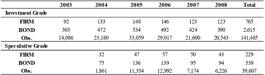
After matching, cleaning, and winsorizing by 1% at the bottom and the top, our final dataset has a total of 181,092 observations. Our final sample covers the period from January 2, 2003, through December 31, 2008. Panel A of Table 1 provides summary information about the firms and bonds in our sample. There are a total of 765 IG firms with 2,615 bonds and 141,485 daily bond observations and 229 HY firms with 539 bonds and 39,607 daily bond observations.
Panel B of Table 1 reports summary statistics for the overall basis (Basis), the predicted basis (Basispredicted), and the residual basis (Basisresidual), as well as a wide range of bond and firm
characteristics. Both Basis and Basispredicted are about –5 basis points, whereas Basisresidual has a
zero mean by construction. Interestingly, both Basis and Basispredicted have a negative mean of –
31 basis points for IG bonds and a positive mean of 81 basis points for HY bonds. Basisresidual has
a zero mean for both IG and HY bonds because we run the cross-sectional regression model for
the IG and HY bonds separately. Basis and Basispredicted tend to have higher standard deviations
14
BBB+ and BBB, an average maturity of 9 years, a coupon rate of 6.6%, and an outstanding amount of $392 million.
Panel C of Table 1 reports the correlation coefficients among all the key variables. We find that the correlation between Basis and Basispredicted is about 0.82. The correlation between Basis
and Basisresidual is about 0.57. We also find that Basisresidual is not highly correlated with all the
control variables, whereas Basispredicted is highly correlated with the past CDS spread (at 0.70)
and credit rating (at 0.54).
3. Empirical Findings
3.1. Predictive Power of the Residual Basis
In this section, we test whether the residual basis has significant predictive power for future bond prices and CDS spreads. In fact, we find that the residual basis predicts price convergence between corporate bonds and CDS. It is important to note that the predictive power is much stronger for bonds than for CDS. The predicted basis, in contrast, exhibits some predictive power for bonds, but not for CDS.
A non-zero residual basis could be due to many factors. For instance, it could reflect the unobservable market frictions and risks encountered in a basis arbitrage, apart from the precision of the model employed to predict the basis. To the extent that our residual basis measure captures mispricing of the unknown limits to arbitrage, one would expect mispricing to narrow in future periods when the limits are not binding, or are less binding.
The arbitrageurs would long (short) bonds with a negative (positive) residual basis, which tend to be underpriced (overpriced) relative to their fundamental values. Since the arbitrage force
15
relation between the residual basis and future bond returns. If the arbitrageurs use CDS to hedge the default risk of the bonds they long or short, then their trading behavior might also affect CDS spreads. The predictive power for each market may differ depending on the degree of mispricing prevalent in the two markets.
We examine the predictive power of the residual and predicted basis for future bond returns and CDS spreads through Fama-MacBeth (1973) regressions with the robust Newey-West (1987) t-statistics for the coefficients with k-1 lags as follows:
, , − , , = + , , + , , + , (5)
∆( ), , − , , = + , , + , , + , , (6)
where HPRi,t,t+kis the k-day holding period return for individual bond i from day t to t+k (where
k=20, 40, or 60), rf,t,t+k is the cumulative risk-free rate from day t to t+k, ∆(CDS)i,t,t+krepresents
the rate of changes in CDS spreads for firm i from day t to t+k, Basisresidual,i,tis the residual basis
on day t, and Basispredicted,i,tis the predicted basis on day t.
The bond control variables in equation (5) include credit rating, maturity, age, coupon, issue
size, and bond liquidity (i.e., turnover) (e.g., Lin, Wang, and Wu, 2011). Following Tang and
Yan (2014), the CDS control variables in equation (6) include Stock Return, the rate of change in
stock price within the past one month; ∆(Volatility), the rate of change of stock volatility within
the past one month (where stock volatility is defined as the standard deviation of daily stock
returns for the past 60-day window); ∆(Leverage), the rate of change in market leverage within
the past three months (where market leverage is defined as the book value of total debt divided
by the market value of total assets); ∆(Size), the rate of change in the logarithm of the market
value of total assets within the past three months; ∆(Profitability), the rate of change in net
16
rate of change in the ratio of cash and cash equivalent divided by the market value of total assets in the past three months.
[Insert Table 2 about Here]
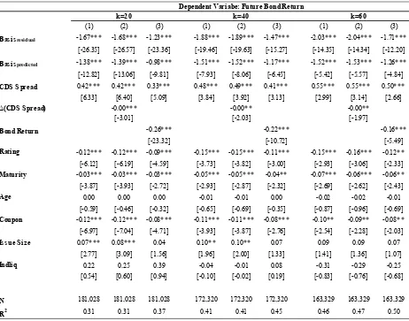
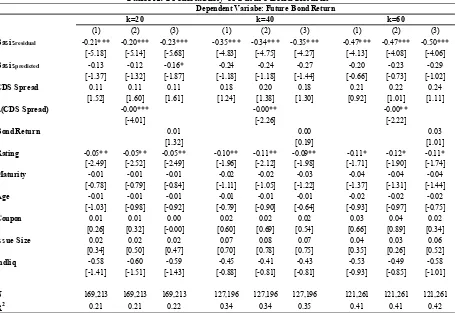
Table 2 reports the regression results for bond excess returns with three different model specifications over 20-, 40-, and 60-day holding horizons. It is shown that the coefficients on
Basisresidual are significantly negative for all bonds at the 1% significance level, ranging from –
2.04 to –1.23 across three different horizons. A one standard deviation decrease in Basisresidual
can generate an annual return of 4.8% to 14.1% for all bonds. These returns would be economically significant after taking into account the high transaction costs in the bond market. Note that the average monthly return of U.S. corporate bonds is about 0.29% according to Barclays U.S. Credit Index from 2003 through 2008 (Barclays Capital, 2010).
Given that the literature has shown that the CDS market is more efficient than the bond market in pricing credit risk (e.g., Zhu, 2004; Blanco, Brennan, and Marsh, 2005; Longstaff, Mithal, and Neis, 2005; Norden and Weber, 2009; Alexopoulou, Andersson, and Georgescu, 2009; Coudert and Gex, 2010), we also control for CDS spreads in the return regression by
including CDS Spread on day t in Table 2. Consistent with the existing literature, we find that
the coefficients of CDS Spread are statistically significant for all bonds at the 1% significance
level. But the coefficient of Basisresidual remains significantly negative for all holding horizons.
We also include lagged bond returns, Bond Return, and changes in CDS spread, Δ(CDS
17
respectively (e.g., Pospisil and Zhang, 2010).9 Bond Return is the lagged individual bond’s
excess return from day t–20 to day t–1. Δ(CDS Spread) is the rate of change in CDS spreads
from day t–20 to day t. The coefficient of Basisresidualremains almost the same in Model 2 but
declines slightly in Model 3. A one standard deviation decrease in Basisresidual can still lead to an
annual return of 4.8% to 10.3% under Model 3. Therefore, these additional control variables do not reduce the strong predictability of the residual basis for future bond returns.
[Insert Table 3 about Here]
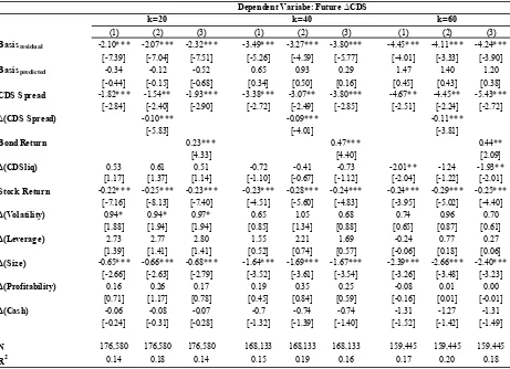
Table 3 reports the regression results for CDS spreads with three different model
specifications over 20-, 40-, and 60-day holding horizons. The predictability of Basisresidual for
future CDS spread changes is very strong and robust: a one standard deviation decrease in
Basisresidual leads to a positive rate of change in CDS spreads of 11.9% to 17.7% on an annual
basis. Models 2 and 3 further control for lagged changes in CDS and bond returns. The coefficients of these additional control variables are significantly negative, indicating that the CDS experience price reversals.
Note in Table 2 and Table 3 that the predictive power of Basispredictedis somewhat limited. It
has highly significant coefficients only for bond returns, but not for CDS spread changes. These results suggest that Basispredicted may capture systematic risk factors, rather than mispricing,
which affects only corporate bonds. As a result, it would predict only bond prices rather than the CDS. Overall, we find that the residual basis predicts subsequent price convergences between corporate bonds and their corresponding CDS.
9 We do not consider including CDS spread, changes in CDS, and bond returns altogether as an explanatory variable
18
3.2. Profitability of a Residual Basis Portfolio
In this section, we first explore whether a convergence trade, a trading strategy that bets on the residual basis getting narrower, can generate significant abnormal returns for corporate bonds. We compute the abnormal returns that can be achieved by investing in corporate bonds using the residual basis as a trading signal. Specifically, we sort bonds into five quintile portfolios based on the residual basis. Next, we long the bottom quintile portfolio with the lowest residual basis and short the top quintile portfolio with the highest residual basis. For comparison, we also compute the returns based on the predicted basis as the trading signal.
To compute the abnormal return of each basis quintile portfolio, we use the following return regression:
, , − , , = , + , , + , , + , ,
+ , , + , , + , , + ,
(7)
where HPRp,t,t+k is the k-day holding period return of the basis portfolio p from day t to t+k
(where k=20), MKT, SMB, and HML are the Fama-French (1993) three factors cumulated daily
from day t to t+k, TERM is the difference between the daily return of the 10-year-to-maturity
government bond index and the daily T-bill return cumulated daily from day t to t+k, DEF is the
difference between the daily return of the Lehman investment-grade bond index and the daily
10-year-to-maturity government bond from CRSP cumulated daily from day t to t+k, and LIQ is the
Amihud (2002) liquidity risk factor measured from day t to t+k by following the procedure in
Lin, Wang, and Wu (2011). Table 4 reports the results.
19
In Panel A of Table 4, we find that the average abnormal returns over the entire sample of the
quintile portfolios of all bonds (which is , in equation (7)) decrease monotonically from 1.58%
to –0.21% for the portfolio with the lowest residual basis to the one with the highest residual basis. If we long the portfolio with the lowest residual basis and short the portfolio with the highest residual basis, we would earn an abnormal return of 1.79% in 20 trading days (2.40% for
a 40-day and 2.68% for a 60-day horizon).10 Edwards, Harris, and Piwowar (2007) show that the
average round-trip cost for a retail order of $20,000 is 1.24%, and the cost decreases to as low as
0.48% for an institutional order of $200,000.11 Hence, the long-short strategy of corporate bonds,
which involves two round-trip transactions, would incur transaction costs of about 2.48% for individuals and 0.96% for institutions. Given that the basis trade is likely to be done by institutional investors with a larger trade size, their take-home profit from the 20-day trading strategy could be approximately 83 basis points net of the transaction cost. The profit will be even larger for longer horizons (144 bps for the 40-day horizon and 172 bps for the 60-day).
In Panel A of Table 4, we also report the yearly breakdown of abnormal returns of the quintile portfolios and reach a similar conclusion, that the low residual basis portfolio has higher returns than the high residual basis portfolio. We also present the abnormal returns of the quintile bond portfolios across various characteristics, such as rating, maturity, age, coupon rate, and
issue size.12 We first sort bonds based on each characteristic, and then on the level of basis on
10 The results for a 40-day and a 60-day horizon are not reported to save the space but are readily available upon
request.
11 The round-trip transaction costs vary within institutional-size trades: 28 bps for a trade size of $500,000 and 18
bps for a trade size of $1M.
12 The details of different bond characteristics considered are as follows: (i) seven rating groups with ratings of AAA,
20
day t. For each portfolio, the value-weighted returns are computed from day t to day t+20. We
find that the long-short strategy earns significant abnormal returns at the 1% significance level across all bond characteristics. The strategy is the most profitable for the oldest bonds and for the bonds with a BBB rating, the longest maturity, the smallest issue size, and higher coupon rates.
Panel B in Table 4 reports parallel results for quintile portfolios sorted by the predicted basis
on day t. Generally, we observe a negative relation between abnormal portfolio returns and the
predicted basis; i.e., the portfolio with the lowest predicted basis has the highest abnormal return. A strategy that longs the portfolio with the lowest predicted basis and shorts the portfolio with the highest predicted basis generally earns a positive abnormal return. The strategy, however, loses money in 2006 and for bonds with extremely high or low credit ratings. More important, the economic significance of the abnormal returns becomes much smaller for the long-short strategy based on the predicted basis.13
In summary, our results show that a long-short strategy based on the residual basis could yield significant abnormal returns across different years and for bond groups with different characteristics. After taking into account the transaction cost, we find that this trading strategy would still generate economically significant returns for institutional investors.
3.3. Profitability of the Negative Basis Trade
In order to exploit the pricing misalignment between corporate bonds and CDS, investors can engage in a popular arbitrage strategy called “negative basis trade”: When the basis is negative,
21
one longs the underlying bond and buys CDS to bet on the narrowing of the basis. Although the positive basis can also allow investors to engage in arbitrage, the negative basis trade is more popular than the positive basis trade because it is difficult to short bonds if the basis is positive. As such, we investigate the profitability of the negative basis trade by buying a very negative CDS-bond basis bond and buying its insurance through CDS for a period (20 days, 40 days, or 60 days) and closing both positions at the end of the period. If the mispricing is corrected, we should expect this arbitrage strategy to generate positive excess returns.
Similar to the analysis in section 3.2, we form the quintile portfolios based on the residual
basis on day t, and measure the realized excess returns from both corporate bonds and CDS for
the next k-day holding period from t to t+k (k=20, 40, and 60). The realized excess returns on CDS are measured by the change in the mark-to-market value of the contract, which is approximated by the multiple of the change in the CDS spread and the value of a default-risky annuity, A(T) (both at T-year maturity):14
, , , = ( , − , ) × ( ) (8)
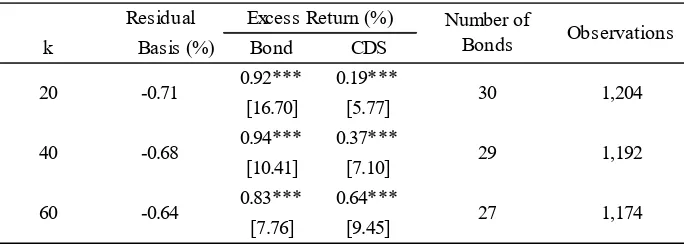
In Table 5, we report the results of excess returns for the quintile portfolio with the most negative basis, which consists of 30 different bonds on average and has an average residual basis of –70 bps. It is shown that our negative basis strategy could generate significant excess returns
14 The value of a risky annuity for CDS of T-year maturity with a quarterly premium payment is computed as
( ) =14 4 4
22
of 1.15% to 1.51% across different investment horizons.15 Overall, these results corroborate our
earlier findings that buying and selling bonds based on non-zero residual basis could generate significant positive trading profits.
[Insert Table 5 about Here]
4. Abnormal Returns of a Residual Basis Portfolio: Risk or Mispricing?
Although the residual basis may capture the temporary price misalignment (i.e., mispricing) of corporate bonds, we perform a more direct test to eliminate the alternative explanation that it may represent a missing systematic risk factor (e.g., Nashikkar, Subrahmanyam, and Mahanti, 2011). Following the standard approach in the literature (e.g., Fama and French, 1993; Daniel and Titman, 1997; Gebhardt, Hvidkjaer, and Swaminathan, 2005), we construct a factor-mimicking portfolio based on the residual basis and test its incremental explanatory power for corporate bond returns over traditional systematic risk factors.
4.1. The Construction of a Residual Basis Factor
We first sort investment-grade (IG) and high-yield (HY) bonds into three groups with low (L),
medium (M), and high (H) levels of the residual basis on day t. Then we construct the
factor-mimicking portfolio for the residual basis as the difference between the average value-weighted 20-day holding period returns of IG and HY bonds with the lowest residual basis (the L group) and for those with the highest residual basis (the H group) (from day t to day t+20), i.e.,
(IG/L+HY/L)/2–(IG/H+HY/H)/2. We name this portfolio the “LMH factor.”
[Insert Table 6 about Here]
15 These returns may be significant, assuming low transaction costs in the CDS market. In fact, Biswas, Nikolova,
23
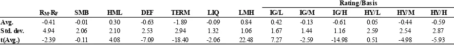
Panel A in Table 6 reports summary statistics of the 20-day returns for the six systematic risk factors (MKT, SMB, HML, DEF, TERM, and LIQ), the LMH factor, and the six portfolios double-sorted by rating and the residual basis. The existing six systematic risk factors are defined in equation (7) and are used in Fama and French (1993) and Lin, Wang, and Wu (2011). Consistent with previous findings, for either the IG or HY category of bond portfolios, the lowest residual basis (the L group) have significantly higher returns than those with the highest residual basis (the H group). The LMH factor has the highest mean return (at 0.84) and the lowest standard deviation (1.06).
Panel B in Table 6 reports the correlation coefficients for all the pricing factors. It shows that the LMH factor is not highly correlated with the other six risk factors. The highest correlation is
with the TERM factor at 0.20. Some of the other factors are significantly correlated with each
other. For example, the correlation between the DEF factor and the MKT factor is 0.79. These
results indicate that the LMH factor may expand the investment opportunity set offered by the existing risk factors. Indeed, Panel C of Table 6 shows that the Sharpe ratio improves substantially from 0.98 in the six-factor model to 1.42 once the LMH factor is included in the optimal portfolio mix.
4.2. Is the LMH Factor a Missing Systematic Risk Factor?
24
, , − , , = , + , , + , , + , , +
, , + , , + , , + ,
(9)
, , − , , = , + , , + , , + , , +
, , + , , + , , + , , + , (10)
where HPRp,t,t+k is the k-day holding period return of bond portfolio p (where p = 6) formed on
bond credit ratings and three basis groups from day t to t+k (where k=20); the systematic risk
factors are defined in equation (7). Panel A in Table 7 provides the results of the six-factor model in equation (9), and Panel B provides the results of the seven-factor model in equation (10).
[Insert Table 7 about Here]
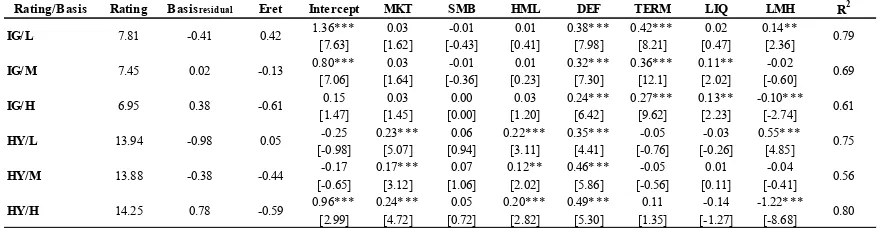
The second and third columns of Panel A in Table 7 reveal a negative relation between the residual basis and portfolio excess returns for IG bonds. It also shows that we have larger return spreads between low and high residual basis portfolios than for HY bonds. The fourth column of Panel A reveals a negative relation between residual basis and portfolio abnormal returns: Portfolios with an extreme low (high) residual basis earn significant positive (negative) abnormal returns, while portfolios with a medium residual basis level (which is closer to zero) earn insignificant excess returns. Moreover, the intercepts are significantly different from zero, especially for IG portfolios under the six-factor model at the 1% significance level. These results suggest that the existing systematic risk factors do not capture the residual basis effect in the average returns.
25
exhibits some co-variations with corporate bond returns, it still cannot completely explain the abnormal returns related to the residual basis.
To further explore whether the LMH factor can explain the return predictability of the residual basis, we apply the seven-factor asset pricing model to 18 triple-sorted bond portfolios, which are constructed based on credit rating (IG and HY), residual basis (L, M, and H), and factor loading on the LMH factor calculated using historical data 180 days prior to portfolio formation (L, M, and H) (i.e., 2×3×3). This approach is adapted from Daniel and Titman (1997). Columns two to four in Panel C of Table 7 show that the triple-sorting leads to portfolios with big variations in the loadings on the LMH factor after controlling for rating and residual basis. However, we do not find a positive relation or any clear pattern between the factor loadings on the LMH factor and the excess returns of the bond portfolios. This indicates that the LMH factor may not represent a missing systematic risk factor. Moreover, the LMH factor is significantly priced in only 11 out of 18 portfolios at the 10% significance level. While a satisfactory asset pricing model should predict zero intercepts for all portfolios, column six shows that 10 out of the 18 portfolios still have significant non-zero intercepts at the 1% significance level. These abnormal returns are economically significant and could be as high as 17.6 percent per annum. These results may suggest that the LMH factor cannot explain the abnormal returns of bond portfolios sorted by the residual basis.
4.3. Risk or Mispricing?
Given that the LMH factor does not explain the abnormal returns related to the residual basis, we run a horse-race between the LMH factor and the residual basis in the return regression as follows,
26
+ , + , + , , + , , + , , + , ,
+ , , + , , + , , + , , + , (11)
where HPRi,t,t+k and rf,t,t+k are defined in the previous regressions; Basisresidual,i,t, RATINGi,t,
Couponi,t, Sizei,t, and Agei,t are the residual basis level, credit rating, coupon rate, issue size, and
age of individual bond i or bond portfolio i on day t, respectively; βMKT,i,t , βSMB,i,t, βHML,i,t, βDEF,i,t,
βTERM,i,t, βLIQ,i,t, and βFLIQ,i,t are the beta loadings on the MKT, SMB, HML, DEF, TERM, LIQ, and
FLIQ factors, respectively; and βLMH,i,t is the beta loading on the LMH factor. These betas are
estimated from day t–180 to day t. The factor MKT, SMB, HML, DEF, TERM, and LIQ are the same systematic risk factors defined in Fama and French (1993) and Lin, Wang, and Wu (2011).
The factor FLIQ is the funding liquidity and is included to control for additional systematic risk
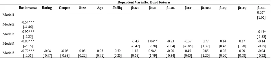
arising from funding constraints (see, e.g., Brunnermeier and Pedersen, 2009). For individual bonds, we also include a liquidity factor (Indliq) that is the sum of the turnover of bond i, which is defined as the total trading volume divided by the total amount outstanding for the bond from day t–20 to day t. We run cross-sectional regressions on each day and report the time-series averages of the estimates of the coefficients in Table 8 (the Fama-Macbeth approach) for both bond portfolios and individual bonds. Robust Newey-West (1987) t-statistics of coefficients are reported in brackets.
[Insert Table 8 about Here]
27
same regression, shows that both coefficients are significantly negative at the 10% significance level. Model 4 includes the loadings of all the existing risk factors, and Model 5 includes all the bond characteristics as specified in equation (11). The coefficient of the residual basis remains significantly negative at the 1% significance level across all these models, whereas that of the LMH factor is not significant at the 10% level. These results suggest that the residual basis captures the mispricing in corporate bonds rather than a missing risk factor.
The results of five parallel models for individual bonds in Panel B of Table 8 are largely similar. They show that the coefficients of the residual basis are significantly negative at the 1% significance level, whereas the coefficients of the LMH factor are only marginally significant at the 5% or 10% significance level. In summary, our regression results provide consistent evidence that the abnormal returns of basis portfolios are more likely due to the mispricing of the bonds.
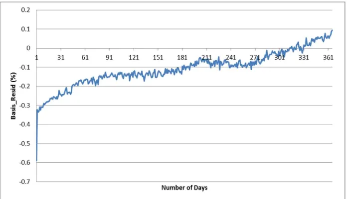
To provide further support for the mispricing interpretation of the abnormal returns from the residual basis portfolio, we examine whether the observed bonds with a highly negative residual basis may experience the convergence of the residual basis subsequently. If the residual basis is due to some missing systematic risk, the residual basis will not necessarily converge to zero. Figure 1 plots the time series of the residual basis for the quintile bond portfolio with the most negative residual basis. For each day, we construct the quintile portfolio based on the residual basis and track the subsequent movement of its residual basis for 300 trading days. We report the average of the residual basis from the formation date to 300 days after. It is shown that the residual basis starts around –60 bps and shrinks by half to –30 bps in one day. The residual basis continues to converge toward zero as time passes. Again, this result indicates that the residual basis is more closely related to mispricing than to an unknown risk factor.
28
5. Robustness Tests
We perform several robustness tests in this section. First, we verify that the predictability of the basis is not driven by a market microstructure issue. Second, we verify that our results are robust for both investment- and speculative-grade bonds and CDS. Third, we confirm that our results are robust even during the recent financial crisis since the literature demonstrates that the credit markets can be disrupted by the limits to arbitrage. Last, we conduct robustness tests using alternative empirical measures for our main variables.
5.1. Microstructure Issue
There is potentially a market microstructure issue when we use the last transaction price of the
day without knowing whether it is a bid price or an ask price.16 Suppose the last transaction on
day t is a trade at the bid price, which is a relatively low price (high yield spread); thus, when
used to compute for the basis, it would have a relatively low (more negative) CDS-bond basis. As this bid price is also used in the computation of future bond returns or the change in CDS
from day t to day t+k, this might create some upward bias in our prediction regression models.
We therefore skip one trading day in constructing the future bond returns and the change in CDS by using the data from day t+1 to day t+k+1. We re-run Table 2 and Table 3 with the new measures and present the results in Table 9 for bond returns (Panel A) and CDS change (Panel B). While there is virtually no change in the results for CDS, the predictability of future bond returns is still statistically significant at the 1% significance level. In economic magnitude, the return predictability is smaller than that in Table 2. A one standard deviation decrease in
Basisresidual is related to an (annualized) excess return of 1.4% to 1.9% under Model 3.
[Insert Table 9 about Here]
29
To confirm that our main result in Table 5 is still robust after taking into account the microstructure issue, we also verify that the negative basis trade is still profitable after skipping one trading day in measuring the returns and the change in CDS. The results are available in Appendix Table A.2.
5.2. Investment and Speculative Grade
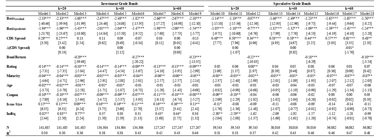
Given that the literature has shown that investment-grade (IG) and high-yield bonds (HY) behave very differently in many dimensions, we perform a subsample analysis on these two groups of bonds separately. For example, Da and Gao (2010) find that the dominant investor clientele for IG and HY bonds are very different from each other. Acharya, Amihud, and Bharath (2013) also show that liquidity of the two types of bonds is very different. Moreover, there is anecdotal evidence that IG bonds are more widely used in basis arbitrage than HY bonds (Deutsche Bank, 2009; Asquith, Au, Covert, and Pathak, 2013). Table 10 reports the results of the subsample analysis of the predictability of the residual basis for future bond returns (Panel A) and CDS spreads (Panel B) in two separate subsamples.
[Insert Table 10 about Here]
Panel A in Table 10 shows that the coefficients of the residual basis are larger for IG bonds than for HY bonds on average (they range from –1.68 to –2.67 for IG bonds and from –0.87 to – 1.65 for HY bonds). This implies that a decrease in Basisresidual will lead to a higher return
30
HY CDS on average (they range from –2.34 to –5.33 for IG and from –1.07 to –1.75 for HY). A
one standard deviation decrease in Basisresidual can lead to about a 20% (12%) change in IG (HY)
CDS spreads for the subsequent 20 trading days. The higher explanatory power in terms of both economic and statistical significance of the basis for investment-grade entities is consistent with the intuition that the investment-grade bonds are more widely used by the basis arbitrageurs.
5.3. Pre-crisis and Crisis Periods
Many studies have shown that the CDS-bond basis experienced dramatic disruption during the recent financial crisis (e.g., Duffie, 2010; Mitchell and Pulvino, 2012). The basis fell into a significantly negative range during the crisis. Table 11 reports the subsample analysis of the predictability of the residual and predicted basis for future bond returns and CDS spreads before and during the crisis. We split the sample into two periods, before the end of June 2007 and after June 2007, when the major U.S. brokerage firm Bear Stearns started to uncover significant losses in its high-grade credit funds.
[Insert Table 11 about Here]
Panel A of Table 11 reports the subsample analysis for corporate bond returns. We find that both the residual and the predicted basis have stronger predictive power for future bond returns before the financial crisis. The coefficients of Basisresidual become smaller during the crisis period
but remain significantly negative at the 1% significance level. The coefficients of Basispredicted
not only decline during the crisis period but also become statistically insignificant when k gets
larger (e.g., when k=40 and 60) at the 10% level. This result reveals again that Basisresidual is
superior to Basispredicted in capturing pure mispricing, since arbitrage force should lead to price
convergence. The risky arbitrage interests (derived from Basispredicted), on the other hand, may
31
the underlying risk during the arbitraging period, which is from day t to t+k. Such a phenomenon
is more likely to occur for a prolonged holding period (when k is bigger) and during the financial
crisis.
Panel B of Table 11 reports the subsample analysis of CDS spreads. First, we find that the residual basis has the stronger predictive power for future CDS spreads before the financial crisis, whereas the predicted basis has almost zero predictability. Second, the predictive power of the residual basis disappeared almost completely during the financial crisis, especially for longer holding horizons. The predicted basis, on the contrary, predicted the positive movement in CDS spread, implying price divergence in the CDS market. These results are consistent with the anecdotal evidence that the CDS market was greatly disrupted during the financial crisis.
We also perform other robustness tests and report these results in the appendix. For example, we report the subsample results for both investment- and speculative-grade credit products for pre-crisis and crisis periods in Appendix Table A.3. We also re-run all the subsample analyses after taking into account the microstructure issues in Appendix Tables A.4, A.5, and A.6. Last, we use different empirical proxies for liquidity risk in Appendix Table A.7. Our main results in Tables 2, 3, and 5 remain robust.
32
arbitrage works better for CDS of IG firms in normal market conditions when the limits to arbitrage are less binding.
6. Conclusion
In this study we document a strong relation between the CDS-bond basis and future bond returns. We find that the residual basis, the part of the CDS-bond basis that cannot be explained by a wide range of known risk factors, captures mispricing between CDS and corporate bonds. Arbitrageurs could achieve significant abnormal returns by buying (shorting) bonds with a low (high) residual basis after controlling for a wide range of systematic factors and bond characteristics. The residual basis strongly predicts price convergence between corporate bonds and CDS, with price adjustments mainly occurring in bond markets. These results suggest that the existence of CDS may help bring the prices of corporate bonds closer to their fundamental values.
33
References
Acharya, Viral, Yakov Amihud, and Sreedhar Bharath, 2013. Liquidity risk of corporate bond
returns: A conditional approach. Journal of Financial Economics 110, 358-386.
Acharya, Viral V. and Lasse Heje Pedersen, 2005. Asset pricing with liquidity risk. Journal of
Financial Economics 77, 375–410.
Alexopoulou, Ioana, Magnus Andersson, and Oana Maria Georgescu, 2009. An empirical study on the decoupling movements between corporate bond and CDS spreads. ECB Working Paper No. 1085.
Amihud, Yakov, 2002. Illiquidity and stock returns: cross-section and time series effects.
Journal of Financial Markets 5, 31–56.
Arora, Navneet, Priyank Gandhi, and Francis A. Longstaff, 2012. Counterparty credit risk and
the credit swap market. Journal of Financial Economics 103, 280–293.
Asquith, Paul, Andrea S. Au, Thomas Covert, and Parag A. Pathak, 2013. The market for
borrowing corporate bonds. Journal of Financial Economics 107, 155–182.
Bai, Jennie and Pierre Collin-Dufresne, 2014. The CDS-Bond basis during the crisis. Working paper, Columbia University.
Baker, Malcolm and Serkan Savasoglu, 2002, Limited arbitrage in mergers and acquisition,
Journal of Financial Economics 64, 91–116.
Bao, Jack and Jun Pan, 2013. Bond illiquidity and excess volatility. Review of Financial Studies
26, 3068–3103.
Bao, Jack, Jun Pan, and Jiang Wang, 2011. The illiquidity of corporate bonds. Journal of
Finance 66, 911–946.
Barclays Capital, 2010. U.S. Credit Index 19 October 2010. Index, portfolio & risk solutions. BIS (Bank for International Settlements), 2010. Credit Risk Transfer Statistics, Bank for International Settlements.
Berndt, Antje and Iulian Obreja, 2010. Decomposing European CDS returns, Review of Finance
34
Biswas, Gopa, Stanislava Nikolova, and Christof W. Stahel, 2015. The Transaction Costs of Trading Corporate Credit. Working Paper, University of Nebraska-Lincoln.
Blanco, Robert, Simon Brennan, and Ian Marsh, 2005. An empirical analysis of the dynamic
relationship between investment grade bonds and credit default swaps. Journal of Finance 60,
2255–2281.
Boehmer, Ekkehart, Sudheer Chava, and Heather E. Tookes, 2013. Related securities and equity
market quality: The case of CDS. Journal of Financial and Quantitative Analysis. Forthcoming.
Bongaerts, Dion, Frank de Jong, and Joost Driessen, 2011. Derivative pricing with liquidity risk:
Theory and evidence from the credit default swap market, Journal of Finance 66, 203-240.
Brunnermeier, Markus K. and Lasse Heje Pedersen, 2009. Market liquidity and funding liquidity.
Review of Financial Studies 22, 2201–2238.
Chen, Long, David Lesmond, and Jason Wei, 2007. Corporate yield spreads and bond liquidity.
Journal of Finance 62, 119–149.
Choudhry, Moorad, 2006. The credit default swap basis. Bloomberg Press, New York.
Coudert, Virginie and Mathieu Gex, 2010. Credit default swap and bond markets: which leads
the other? Financial Stability Review No.14 – Derivatives – Financial Innovations and Stability,
161–167.
Da, Zhi, and Pengjie Gao, 2010. Clientele change, liquidity shock, and the return on financially
distressed stock. Journal of Financial and Quantitative Analysis 45, 27-48.
Daniel, Kent, and Sheridan Titman, 1997. Evidence on the characteristics of cross sectional
variation in common stock returns, Journal of Finance 52, 1–33.
Das, Sanjiv, Madhu Kalimipalli, and Subhankar Nayak, 2014. Did CDS trading improve the
market for corporate bonds? Journal of Financial Economics 111, 495-525.
Deutsche Bank, 2009. CDS-bond basis update, quantitative credit strategy, Global Markets Research.
Dick-Nielsen, Jens, Peter Feldhütter, and David Lando, 2012. Corporate bond liquidity before
35
Duffie, Darrell, 2010. Presidential address: asset pricing dynamics with slow-moving capital.
Journal of Finance 65, 1237–1267.
Edwards, Amy K., Harris E. Lawrence, and Michael S. Piwowar, 2007. Corporate bond market
transaction costs and transparency. Journal of Finance 62, 1421–1451.
Fama, Eugene and Kenneth French, 1993. Common risk factors in the returns of stocks and
bonds. Journal of Financial Economics 33, 3–56.
Fama, Eugene and James MacBeth, 1973. Risk, return and equilibrium: empirical tests. Journal
of Political Economy 81, 607–636.
Fleckenstein, Matthias, Francis A. Longstaff, and Hanno Lustig, 2014, The Tips-Treasury Bond
Puzzle, Journal of Finance 69, 2151–2197.
Fontana, Alessandro, 2011. The persistent negative CDS-bond basis during the 2007–08 financial crisis. Working paper, University of Venice, Italy, unpublished.
Fontana, Alessandro, and Martin Scheicher, 2010. An analysis of euro area sovereign CDS and their relation with government bonds, Working paper, European Central Bank.
Friewald, Nils, Rainer Jankowitsch, and Marti G. Subrahmanyam, 2012. Illiquidity or credit deterioration: a study of liquidity in the US corporate bond market during financial crisis.
Journal of Financial Economics 105, 18–36.
Gebhardt, William, Soeren Hvidkjaer, and Bhaskaran Swaminathan, 2005. The cross-section of
expected corporate bond returns: betas or characteristics? Journal of Financial Economics 75,
85–114.
Goldstein, Michael A., Edith S. Hotchkiss, and Erik R. Sirri, 2007. Transparency and liquidity: a
controlled experiment on corporate bonds. Review of Financial Studies 20, 235–273.
JP Morgan, 2006. Credit derivative handbook. Corporate Quantitative Research.
Kim, Gi H., Haitao Li, and Weina Zhang, 2013. The CDS-Bond basis arbitrage and the cross-section of corporate bond returns. Working Paper, National University of Singapore.
36
Lee, Charles M.C., James Myers, and Bhaskaran Swaminathan, 1999. What is the intrinsic value
of the Dow? Journal of Finance, 54(5), 1693-1741.
Lin, Hai, Junbo Wang, and Chunchi Wu, 2011. Liquidity risk and the cross-section of expected
corporate bond returns. Journal of Financial Economics 99, 628–650.
Longstaff, Francis, Sanjay Mithal, and Eric Neis, 2005. Corporate yield spreads: default risk or
liquidity? New evidence from the credit default swap market. Journal of Finance 60, 2213–2253.
Mitchell, Mark and Todd Pulvino, 2012. Arbitrage crashes and the speed of capital. Journal of
Financial Economics 104, 469–490.
Mitchell, Mark, Todd Pulvino, and Erik Stafford, 2002. Limited Arbitrage in Equity Markets,
Journal of Finance 57, 551–584.
Nashikkar, Amrut, Marti G. Subrahmanyam, and Sriketan Mahanti, 2011. Liquidity and
arbitrage in the market for credit risk. Journal of Financial and Quantitative Analysis 46, 627–
656.
Newey, Whitney and Kenneth West, 1987. A simple, positive definite, heteroskedasticity and
autocorrelation consistent covariance matrix. Econometrica 55, 703–708.
Norden, Lars and Martin Weber, 2009. The co-movement of credit default swap, bond and stock
markets: an empirical analysis. European Financial Management 15, 529–562.
Pástor, Lubos , and Robert F. Stambaugh, 2003. Liquidity risk and expected stock returns.
Journal of Political Economy 111, 642–685.
Pospisil, Libor, and Jing Zhang, 2010. Momentum and reversal effects in corporate bond prices
and credit cycles. Journal of Fixed Income 20, 101–115.
Shleifer, Andrei and Robert W. Vishny, 1997. The limits to arbitrage. Journal of Finance 52,
35–55.
Tang, Dragon Yongjun and Yan Hong, 2014. Liquidity and credit default swap spreads. Working paper, The University of Hong Kong.
37
38
Figure 1. Time Series of Residual Basis for the Most Negative Basis Bonds
39
Table 1. Summary Statistics
This table provides summary statistics about the sample firms and bonds used in the analysis from 2003 through 2008. Panel A reports the yearly breakdown of the number of firms and bonds for investment-grade and high-yield bonds. Panel B reports summary statistics for the key variables. Panel C reports the correlation coefficient matrix of these variables with the statistically significant numbers in gray. Basis is defined as (CDS spread – Z-spread) on day
t for the individual bond. Basispredictedis the predicted component of Basis by the model in Bai and Collin-Dufresne (2014), and Basisresidual is computed as (Basis – Basispredicted). Bond Return is the individual bond’s 20-day excess return from day t–20 to day t. CDS Spread is the CDS spread on day t and Δ(CDS Spread) is the rate of CDS spread changes from day t–20 to day t. Rating is a categorical variable ranging from 1 to 20 for all bonds (S&P rating AAA to CC). We use the S&P ratings whenever available, followed by Moody’s and Fitch’s ratings. Coupon is in percentage terms. Issue size is the natural logarithm of the issuance amount in billions. Maturity and age are in years.
Indliq is the 20-day cumulative turnover measured as the total trading volume divided by the total number outstanding. Δ(CDSliq) is the 20-day change in the number of CDS dealers’ quotes. Stock return is the rate of changes in stock prices within the past one month. Δ(Volatility) is the rate of change in stock volatility within the past one month, where stock volatility is defined as the standard deviation of daily stock returns measured in a 60-day window. Δ(Leverage) is the rate of change in market leverage within the past three months, where market leverage is measured by the book value of total debt divided by the market value of total assets. Δ(Size) is the rate of change in the logarithm of the market value of total assets within the past three months. Δ(Profitability) is the rate of change in net income divided by the market value of total assets within the past three months. Δ(Cash) is defined as the rate of change in the cash ratio in the past three months. The cash ratio is defined as the ratio of cash and cash equivalent divided by the market value of total assets.
Panel A: Yearly Breakdown of the Number of Firms and Bonds
2003 2004 2005 2006 2007 2008 Total Investment Grade
FIRM 92 133 148 146 123 123 765
BOND 303 472 534 492 424 390 2,615
Obs. 14,086 23,180 33,059 29,017 21,600 20,543 141,485
Speculative Grade
FIRM 32 47 57 50 43 229
BOND 75 136 139 95 94 539
40
Panel B: Summary Statistics
N MEAN STD MIN MAX Basis (% ) 181,092 -0.05 1.02 -3.30 8.28
Basispredicted 181,092 -0.05 0.84 -4.16 8.44
Basisresidual 181,092 0.00 0.58 -6.77 6.12
Investment Grade
Basis 141,485 -0.30 0.55 -3.30 0.98 Basispredicted 141,485 -0.30 0.40 -3.56 3.37
Basisresidual 141,485 0.00 0.39 -3.00 2.96
Speculative Grade
Basis 39,607 0.81 1.66 -3.30 8.28
Basispredicted 39,607 0.81 1.32 -4.16 8.44
Basisresidual 39,607 0.00 1.01 -6.77 6.12
Bond Return (% ) 181,092 0.03 2.63 -9.51 8.40
CDS Spread (% ) 181,092 1.53 2.81 0.02 55.65 ∆(CDS Spread) (% ) 181,092 1.83 20.68 -39.22 89.85 Rating 181,092 8.59 3.61 1.00 20.00
Maturity 181,092 9.08 7.66 1.04 29.94
Issue Size 181,092 12.88 0.58 10.82 14.51
Age 181,092 5.72 4.09 0.05 26.06
Coupon 181,092 6.57 1.42 1.95 11.25
Indliq 181,028 0.05 0.06 0.00 1.16
∆(CDSliq) 180,850 0.00 0.32 -1.95 1.79
Stock Return (% ) 176,465 0.24 9.27 -75.58 172.48 ∆(Volatility) 176,871 0.10 0.47 -0.96 6.32 ∆(Leverage) 178,955 0.02 0.84 -0.93 191.99
∆(Size) (% ) 178,956 0.08 1.32 -12.21 11.37
41
Panel C: Correlation Coefficients
(1) (2) (3) (4) (5) (6) (7) (8) (9) (10) (11) (12) (13) (14) (15) (16) (17) (18)
(1) Basis 1.00
(2) Basispredicted 0.82 1.00
(3) Basisresidual 0.57 0.00 1.00 (4) Bond Return 0.10 0.02 0.16 1.00 (5) CDS Spread 0.69 0.70 0.19 -0.11 1.00 (6) ∆(CDS Spread) -0.01 -0.03 0.03 -0.22 0.09 1.00 (7) Rating 0.44 0.54 0.00 0.00 0.67 -0.01 1.00 (8) Maturity -0.08 -0.01 -0.12 -0.01 0.09 0.02 0.04 1.00
(9) Age 0.07 0.10 -0.03 0.00 0.16 0.00 0.09 0.09 1.00