University of Warwick institutional repository: http://go.warwick.ac.uk/wrap
A Thesis Submitted for the Degree of PhD at the University of Warwick
http://go.warwick.ac.uk/wrap/59744
This thesis is made available online and is protected by original copyright.
Please scroll down to view the document itself.
Library Declaration and Deposit Agreement
1. STUDENT DETAILS
Please complete the following:
Full name: ………. University ID number: ………
2. THESIS DEPOSIT
2.1 I understand that under my registration at the University, I am required to deposit my thesis with the University in BOTH hard copy and in digital format. The digital version should normally be saved as a single pdf file.
2.2 The hard copy will be housed in the University Library. The digital version will be deposited in the University’s Institutional Repository (WRAP). Unless otherwise indicated (see 2.3 below) this will be made openly accessible on the Internet and will be supplied to the British Library to be made available online via its Electronic Theses Online Service (EThOS) service.
[At present, theses submitted for a Master’s degree by Research (MA, MSc, LLM, MS or MMedSci) are not being deposited in WRAP and not being made available via EthOS. This may change in future.] 2.3 In exceptional circumstances, the Chair of the Board of Graduate Studies may grant permission for an embargo to be placed on public access to the hard copy thesis for a limited period. It is also possible to apply separately for an embargo on the digital version. (Further information is available in the Guide to Examinations for Higher Degrees by Research.)
2.4 If you are depositing a thesis for a Master’s degree by Research, please complete section (a) below. For all other research degrees, please complete both sections (a) and (b) below:
(a) Hard Copy
I hereby deposit a hard copy of my thesis in the University Library to be made publicly available to readers (please delete as appropriate) EITHER immediately OR after an embargo period of ………... months/years as agreed by the Chair of the Board of Graduate Studies. I agree that my thesis may be photocopied. YES / NO (Please delete as appropriate)
(b) Digital Copy
I hereby deposit a digital copy of my thesis to be held in WRAP and made available via EThOS. Please choose one of the following options:
EITHER My thesis can be made publicly available online. YES / NO(Please delete as appropriate)
OR My thesis can be made publicly available only after…..[date] (Please give date)
YES / NO(Please delete as appropriate)
OR My full thesis cannot be made publicly available online but I am submitting a separately identified additional, abridged version that can be made available online.
YES / NO (Please delete as appropriate)
OR My thesis cannot be made publicly available online. YES / NO(Please delete as appropriate)
Xin Lu
Rights granted to the University of Warwick and the British Library and the user of the thesis through this agreement are non-exclusive. I retain all rights in the thesis in its present version or future versions. I agree that the institutional repository administrators and the British Library or their agents may, without changing content, digitise and migrate the thesis to any medium or format for the purpose of future preservation and accessibility.
4. DECLARATIONS
(a) I DECLARE THAT:
I am the author and owner of the copyright in the thesis and/or I have the authority of the authors and owners of the copyright in the thesis to make this agreement. Reproduction of any part of this thesis for teaching or in academic or other forms of publication is subject to the normal limitations on the use of copyrighted materials and to the proper and full acknowledgement of its source.
The digital version of the thesis I am supplying is the same version as the final, hard-bound copy submitted in completion of my degree, once any minor corrections have been completed.
I have exercised reasonable care to ensure that the thesis is original, and does not to the best of my knowledge break any UK law or other Intellectual Property Right, or contain any confidential material.
I understand that, through the medium of the Internet, files will be available to automated agents, and may be searched and copied by, for example, text mining and plagiarism detection software.
(b) IF I HAVE AGREED (in Section 2 above) TO MAKE MY THESIS PUBLICLY AVAILABLE DIGITALLY, I ALSO DECLARE THAT:
I grant the University of Warwick and the British Library a licence to make available on the Internet the thesis in digitised format through the Institutional Repository and through the British Library via the EThOS service.
If my thesis does include any substantial subsidiary material owned by third-party copyright holders, I have sought and obtained permission to include it in any version of my thesis available in digital format and that this permission encompasses the rights that I have granted to the University of Warwick and to the British Library.
5. LEGAL INFRINGEMENTS
I understand that neither the University of Warwick nor the British Library have any obligation to take legal action on behalf of myself, or other rights holders, in the event of infringement of intellectual property rights, breach of contract or of any other right, in the thesis.
Please sign this agreement and return it to the Graduate School Office when you submit your thesis.
Video Coding
Xin Lu, BEng, MSc.
A thesis submitted in partial fulfilment of the requirements for the degree of Doctor of Philosophy in Computer Science
List of Figures v
List of Tables viii
Acknowledgement x
Dedication xi
Declaration xii
Publications xiii
Abstract xiv
Abbreviations xv
1 Introduction 1
1.1 Fundamental Techniques in Video Compression . . . 2
1.1.1 Predictive Coding . . . 3
1.1.2 Transforms and Quantisation . . . 6
1.1.3 Entropy Coding . . . 10
1.2 International Video Coding Standards . . . 13
1.2.2 ISO/IEC MPEG-1, MPEG-2, and MPEG-4 Visual . . . 16
1.2.3 ITU-T H.264/MPEG-4 AVC . . . 19
1.2.4 ITU-T H.265/MPEG-H HEVC . . . 20
1.3 Research Contributions . . . 23
1.4 Thesis Outline . . . 24
2 Scalable Video Coding 26 2.1 Overview of the Scalable Extension of H.264/AVC . . . 27
2.1.1 Structure . . . 28
2.1.2 Basic Modes of Scalability . . . 30
2.2 Coding Methods . . . 37
2.2.1 Prediction . . . 38
2.2.2 DCT Transform and Quantisation . . . 44
2.2.3 Entropy Coding . . . 46
2.3 Coding Mode Decisions . . . 49
2.3.1 Rate Distortion Optimisation . . . 49
2.3.2 Computational Complexity Analysis . . . 51
2.4 Rate Control . . . 54
2.5 Summary . . . 56
3 Performance Evaluation of Advanced Scalable Video Coding Schemes 58 3.1 Introduction . . . 59
3.1.1 Motion JPEG2000 . . . 60
3.1.2 Wavelet Scalable Video Coding . . . 69
3.2 Performance Evaluation Design . . . 74
3.2.1 Video Test Sequences . . . 74
3.2.2 Codec Settings . . . 75
3.3 Results and Discussions . . . 76
3.3.1 Evaluations for Low and Medium Resolution Video . . . 76
3.3.2 Evaluations for High Resolution Video . . . 80
3.4 Summary . . . 84
4 Fast Mode Decisions Based on Motion Activity 85 4.1 Existing SVC Fast Algorithms . . . 86
4.1.1 Fast Algorithms Extended from Single Layer Coding . . . 87
4.1.2 Solutions Targeting Inter-layer Prediction . . . 88
4.2 The Proposed Fast Mode Decision Algorithm . . . 89
4.2.1 Observations and Algorithm Formulation . . . 90
4.2.2 Algorithm Description . . . 95
4.3 Simulations, Comparisons, and Discussion . . . 98
4.3.1 Simulation Results for Various Values of Qp . . . 99
4.3.2 RD Comparison with the JSVM Implementation . . . 101
4.4 Summary . . . 105
5 Hierarchical Scheme for Fast Mode Decisions 107 5.1 Introduction . . . 108
5.2 The Proposed Hierarchical Mode Decision Scheme . . . 109
5.2.1 Observations, Analysis, and Algorithm Formulation . . . 109
5.2.2 The Structure of the Proposed Algorithm . . . 118
5.3 Simulations, Comparisons, and Discussion . . . 121
5.3.1 Simulation Results for Various Values of Qp . . . 121
5.3.2 Overall Comparison with the JSVM Implementation . . . 124
5.3.3 Comparisons with Other Algorithms . . . 128
6 Improved Rate Control Scheme for SVC 132
6.1 Existing Rate Control Algorithms . . . 133
6.1.1 Default Implementation in JSVM . . . 133
6.1.2 Other Improved Algorithms . . . 135
6.2 The Proposed Rate Control Algorithm . . . 137
6.2.1 RD Models for Prediction Modes . . . 137
6.2.2 Optimisation of the MAD Prediction Model . . . 143
6.2.3 Overall Structure of the Proposed Algorithm . . . 151
6.3 Simulations, Comparisons, and Discussion . . . 152
6.3.1 MAD Prediction Accuracy . . . 153
6.3.2 Rate Control Accuracy and RD Performance . . . 155
6.4 Summary . . . 167
7 Conclusions and Further Work 168 7.1 Performance Comparison of Advanced Scalable Video Coding Schemes . . . 169
7.2 Fast Algorithms for SVC . . . 170
7.2.1 Fast Inter-frame and Inter-layer Mode Decisions . . . 170
7.2.2 Hierarchical Scheme for Fast Mode Selection . . . 173
7.3 Rate Control for SVC with Optimised RD Model . . . 175
7.4 Directions for Further Work . . . 176
7.4.1 Fast Algorithms for HEVC . . . 177
7.4.2 Rate Control for HEVC . . . 178
7.5 Concluding Remarks . . . 178
1-1 4:2:0 chrominance component subsampling. . . 2
1-2 I-, P- and B-frames in a Group of Pictures (GOP). . . 4
1-3 Block diagram of a typical predictive codec. . . 5
1-4 An example of the forward DCT transform. . . 8
1-5 Uniform quantisers. . . 10
1-6 Quantisation results with quantisation step sizeQs=8. . . 11
1-7 Zig-zag scan of quantisation coefficients. . . 12
1-8 Progression of the international video coding standards. . . 13
1-9 Block diagram of a typical H.261 video encoder. . . 15
2-1 Scalable video coding over heterogeneous networks with heterogeneous terminals. . . 28
2-2 The general coding structure of the scalable extension of H.264/AVC with three spatial layers. . . 29
2-3 Temporal scalability with three temporal decomposition levels. . . 31
2-4 Spatial scalability with two spatial layers. . . 33
2-5 Quality scalable structure in MGS. . . 35
2-6 Hybrid scalability with two spatial layers. . . 37
2-7 Nine prediction patterns of intra 4×4 type. . . 38
2-9 Inter-layer motion prediction in SVC. . . 41
2-10 Inter-layer residual prediction in SVC. . . 42
2-11 Inter-layer intra-prediction in SVC. . . 43
2-12 Block diagram of a CAVLC encoder. . . 47
2-13 Block diagram of a CABAC encoder. . . 48
2-14 Rate distortion function. . . 49
2-15 Encoding time comparison of different encoding options. . . 53
2-16 Bit rate fluctuation. . . 54
3-1 General framework for a JPEG2000 encoder. . . 61
3-2 Two level 2D wavelet decomposition of image ‘Woman’. . . 62
3-3 Convolution implementation of the wavelet transform. . . 64
3-4 Lifting implementation of the wavelet transform. . . 65
3-5 Scalar quantiser with quantisation step size4b and a 24b wide dead zone. 66 3-6 An 8 bit image that is composed of 8 bit planes ranging from LSB to MSB. . . 67
3-7 Block diagram of an EBCOT tier-1 encoder. . . 68
3-8 Fundamental framework of WSVC. . . 69
3-9 Motion-compensated temporal decomposition using Haar wavelet. . . 70
3-10 Wavelet transform using the CDF 9/7 lifting scheme. . . 72
3-11 Embedded dead zone uniform scalar quantiser. . . 72
3-12 RD performance for low and medium resolution video sequences. . . 78
3-13 RD performance for high resolution video sequences. . . 82
4-1 A typical hierarchical B-frame coding structure. . . 91
4-2 An example of a linear motion trajectory. . . 92
4-3 MVs of a current block and its neighbours. . . 93
4-4 Inter-layer MV prediction with various block sizes. . . 94
4-6 Overall flowchart of the proposed algorithm. . . 96
4-7 Relationship between P-frame MVD values and the percentage of SKIP_MODE decisions when an exhaustive evaluation is conducted. . . 97
4-8 RD performance comparison of JSVM and the proposed algorithm. . . 103
5-1 Spatial locations of neighbouring macroblocks in the same layer and co-located macroblock in the base layer. . . 112
5-2 Relationship between AC energy threshold and both prediction accuracy and computational time reduction. . . 116
5-3 Relationship between MVD threshold and both prediction accuracy and computational time reduction. . . 118
5-4 Overall scheme of proposed hierarchical algorithm. . . 120
5-5 Encoding time for video sequences for various Qp values. . . 123
5-6 RD performance for different video sequences. . . 125
6-1 Relationship between average number of bits andQstepfor both inter-layer coding and intra-layer coding. Points are actual data; curves are fitted to the data. . . 140
6-2 Relationship between predicted and actual MAD values. . . 145
6-3 Relationship between actual MAD values of base layer and those of the spatial enhancement layer. . . 146
6-4 Overall scheme of proposed algorithm. . . 150
6-5 RD performance for QCIF/CIF video sequences. . . 161
6-6 RD performance for CIF/4CIF video sequences. . . 163
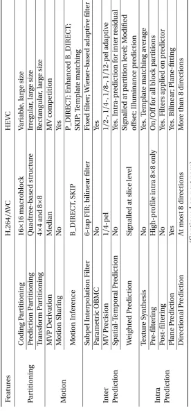
1-1 Comparison of tools in H.264/MPEG-4 AVC and H.265/MPEG-H HEVC . . . 21
2-1 Other macroblock prediction modes in SVC . . . 43
2-2 Qp and its corresponding quantisation step sizeQstep. . . 45
2-3 Multiplication factor MF for scaling function . . . 46
3-1 Core algorithms in each coding scheme . . . 60
3-2 Daubechies 9/7 LPF and HPF coefficients for analysis and synthesis filters . 63 3-3 Le Gall 5/3 LPF and HPF coefficients for analysis and synthesis filters . . . 63
3-4 Video test sequences used for evaluation . . . 75
3-5 RD performance for low and medium resolution video sequences . . . 77
3-6 RD performance for high resolution video sequences . . . 81
4-1 % Percentage of SKIP_MODE decisions made for different P-frame MVD values . . . 97
4-2 Computational performance for ‘Bus’ sequence . . . 100
4-3 Computational performance for ‘Foreman’ sequence . . . 100
4-4 Computational performance for ‘Mobile’ sequence . . . 101
4-5 Computational performance for ‘Mother-daughter’ sequence . . . 101
4-6 Overall comparison of proposed algorithm and JSVM implementation . . . . 102
5-1 % Mode correlation between base layer and corresponding enhancement
layer . . . 111
5-2 % Mode correlation between macroblock and its neighbours . . . 113
5-3 % Prediction accuracy and time reduction corresponding to different AC energy thresholds . . . 116
5-4 % Prediction accuracy and time reduction corresponding to different MVD thresholds . . . 118
5-5 Performance when encoding QCIF/CIF sequences . . . 122
5-6 Overall comparison of proposed algorithm and JSVM implementation . . . . 124
5-7 Performance when encoding CIF/4CIF sequences . . . 127
5-8 Performance when encoding QCIF/CIF/4CIF sequences . . . 128
5-9 Comparison of proposed algorithm with Kim’s algorithm . . . 129
5-10 Comparison of proposed algorithm with Zhao’s algorithm . . . 129
5-11 Comparison of proposed algorithm with Lee’s algorithm . . . 130
6-1 Average number of bits per macroblock for both inter-layer predicted macroblocks and intra-layer predicted macroblocks . . . 139
6-2 MAD correlation between base layer and corresponding enhancement layer 147 6-3 MAD prediction accuracy comparison for spatial enhancement layer . . . 154
6-4 Comparison of proposed algorithm with JVT-W043 when encoding QCIF/CIF sequences . . . 157
6-5 Comparison of proposed algorithm with JVT-W043 when encoding CIF/4CIF sequences . . . 158
First and foremost, I would like to take this opportunity to express my deepest gratitude and respect to my supervisor Dr. Graham Martin, who constantly
of-fered fruitful guidance and strong support during all the time that I was in the
Department of Computer Science at the University of Warwick. I benefitted greatly from his insightful advice, continuous encouragement and generous
help and cannot help feeling lucky to be able to work with him. I am also
look-ing forward to maintainlook-ing our collaboration in the future.
My parents, Lu Wenting and Wei Guangxian, and sister, Lu Na, also deserve cordial gratitude. Their love, support and encouragement have always been
the source of my strength and the reason I have progressed this far. In
par-ticular, my wife, Gu Qian has unconditionally supported me throughout my studies at Warwick. Her selfless care, dedication, and love are my most
valu-able assets.
I also want to thank my friends and colleagues at Warwick, particularly Chen
Chao, Gao Bo, Li Ruizhe, Xia Weixi, and Zhu Huanzhou for their support and friendship. They made life on the campus at Warwick enjoyable and joyful.
Last, but not least I wish to express my sincere thanks to my friend Jin Xuesong
for his generous help and beneficial advice. I have benefitted a lot from his
I hereby declare that, except where acknowledged, the work presented in this thesis is my own work. No part of the work contained in this thesis has
previ-ously been accepted in substance for any degree nor submitted elsewhere for
the purpose of obtaining an academic degree.
Xin Lu
Signature:
1. X. Lu, G. Martin, “Performance comparison of the SVC, WSVC, and Motion JPEG2000 advanced scalable video coding schemes,” accepted for
publica-tion inProc. IET Intelligent Signal Process., 6pp., Dec. 2013.
2. X. Lu, G. Martin, and X. Jin, “An improved rate control algorithm for SVC with optimised MAD prediction,” inProc. York Doctoral Symposium (YDS 2013), 1pp., Oct. 2013.
3. X. Lu, G. Martin, “Rate control for scalable video coding with rate-distortion analysis of prediction modes,” inProc. IEEE Multimedia Signal Process., pp. 289-294, Sep. 2013.
4. X. Lu, G. Martin, “Fast implementation of the scalable video coding exten-sion of the H.264/AVC standard,” inProc. Imperial College Computing Stu-dent Workshop (ICCSW’13), pp. 65-72, Sep. 2013.
5. X. Lu, G. Martin, “Improved rate control algorithm for scalable video cod-ing,” inProc. Imperial College Computing Student Workshop (ICCSW’13), pp. 73–81, Sep. 2013.
6. X. Lu, G. Martin, “Fast mode decision algorithm for the H.264/AVC scalable video coding extension,”IEEE Trans. Circuits Syst. Video Technol. vol.23, no.5, pp. 846-855, May 2013.
7. X. Lu, G. Martin, “A hierarchical mode decision scheme for fast
implemen-tation of spatially scalable video coding,” inProc. IEEE Visual Commun. Image Process., pp. 1-6, Nov. 2012.
8. X. Lu, “A improved scheme for fast implementation of scalable video
cod-ing and the performance comparison of advanced image codcod-ing schemes”
Technical Report, University of Warwick, Jul. 2012.
9. X. Lu, G. Martin, “Fast H.264/SVC inter-frame and inter-layer mode
deci-sions based on motion activity,”IET Electron. Lett., vol.48, no.2, pp. 84-86, Jan. 2012.
10. X. Lu, “Novel schemes for fast implementation of scalable video coding,”
The University of Warwick For the degree of Doctor of Philosophy
September 2013
Summary
A scalable video bitstream specifically designed for the needs of various client terminals, network conditions, and user demands is much desired in current and future video trans-mission and storage systems. The scalable extension of the H.264/AVC standard (SVC) has been developed to satisfy the new challenges posed by heterogeneous environments, as it permits a single video stream to be decoded fully or partially with variable quality, res-olution, and frame rate in order to adapt to a specific application. This thesis presents novel improved algorithms for SVC, including: 1) a fast inter-frame and inter-layer coding mode selection algorithm based on motion activity; 2) a hierarchical fast mode selection algorithm; 3) a two-part Rate Distortion (RD) model targeting the properties of different prediction modes for the SVC rate control scheme; and 4) an optimised Mean Absolute Difference (MAD) prediction model.
The proposed fast inter-frame and inter-layer mode selection algorithm is based on the empirical observation that a macroblock (MB) with slow movement is more likely to be best matched by one in the same resolution layer. However, for a macroblock with fast movement, motion estimation between layers is required. Simulation results show that the algorithm can reduce the encoding time by up to 40%, with negligible degradation in RD performance.
The proposed hierarchical fast mode selection scheme comprises four levels and makes full use of inter-layer, temporal and spatial correlation as well as the texture information of each macroblock. Overall, the new technique demonstrates the same coding performance in terms of picture quality and compression ratio as that of the SVC standard, yet produces a saving in encoding time of up to 84%. Compared with state-of-the-art SVC fast mode selection algorithms, the proposed algorithm achieves a superior computational time re-duction under very similar RD performance conditions.
The existing SVC rate distortion model cannot accurately represent the RD properties of the prediction modes, because it is influenced by the use of inter-layer prediction. A sep-arate RD model for inter-layer prediction coding in the enhancement layer(s) is therefore introduced. Overall, the proposed algorithms improve the average PSNR by up to 0.34dB or produce an average saving in bit rate of up to 7.78%. Furthermore, the control accuracy is maintained to within 0.07% on average.
As a MAD prediction error always exists and cannot be avoided, an optimised MAD predic-tion model for the spatial enhancement layers is proposed that considers the MAD from previous temporal frames and previous spatial frames together, to achieve a more accu-rate MAD prediction. Simulation results indicate that the proposed MAD prediction model reduces the MAD prediction error by up to 79% compared with the JVT-W043 implemen-tation.
2D Two-Dimensional
3D Three-Dimensional
3DTV Three-Dimensional Television AC Alternating Current (high frequency)
AVC Advanced Video Coding
B-frame Bi-directional predictive-coded frame BDBR Bjφntegaard Bit Rate
BDPSNR Bjφntegaard PSNR
BL Base Layer
BLMVP Base Layer Motion Vector Predictor
BPC Bit Plane Coder
BR Bit Rate
CABAC Context-Adaptive Binary Arithmetic Coding CAVLC Context-Adaptive Variable Length Coding
CBR Constant Bit Rate
CCF Cross-Correlation Function CCTV Closed-Circuit Television
CD-ROM Compact Disc Read-Only Memory
CDF Cohen-Daubechies-Feauveau
CGS Coarse Grain Scalability
CIF Common Intermediate Format
CUP Cleanup Pass
DC Direct Current (lowest frequency) DCT Discrete Cosine Transform DFT Discrete Fourier Transform
DHT Discrete Hadamard Transform
DPCM Differential Pulse-Code Modulation
DST Discrete Sine Transform
EBCOT Embedded Block Coding with Optimised Truncation
EL Enhancement Layer
EOB End-of-Block
ESCOT Embedded Subband Coding with Optimal Truncation FGS Fine Grain Scalability
fps frames per second
GOP Group of Pictures
HD High Definition
HDTV High Definition Television HEVC High Efficiency Video Coding HHI Heinrich Hertz Institute
HM HEVC Test Model
HPF High-Pass FIR Filter
HVS Human Visual System
I-frame Intra-coded frame
IDCT Inverse Discrete Cosine Transformation IDR Instantaneous Decoding Refresh
IEC International Electrotechnical Commission IPTV Internet Protocol Television
ISDN Integrated Services Digital Network ISO International Standards Organisation
ITU-T International Telecommunications Union Telecommunication Standardisation Sector
JCT-VC Joint Collaborative Team on Video Coding JPEG Joint Photographic Experts Group
JSVM Joint Scalable Video Model JTC1 Joint Technical Committee 1
JVT Joint Video Team
KLT Karhunen Loève Transform
LPF Low-Pass FIR Filter
LSB Least Significant Bit
MAD Mean Absolute Difference
MAE Mean Absolute Error
MB Macroblock
MCTF Motion-Compensated Temporal Filtering MGS Medium Grain Scalability
MPEG Moving Picture Experts Group
MRC Magnitude Refinement Coding
MRP Magnitude Refinement Pass
MSB Most Significant Bit
MSE Mean Squared Error
MSRA Microsoft Research Asia
MVD Motion Vector Difference
MVP Motion Vector Predictor
P-frame Predictive-coded frame
PA Prediction Accuracy
PCC Pearson Correlation Coefficient PSNR Peak Signal-to-Noise Ratio
PSTN Public Switched Telephone Network QCIF Quarter Common Intermediate Format
Qp Quantisation Parameter
R-Q Rate-Quantisation
RD Rate Distortion
RDO Rate Distortion Optimisation
RLC Run Length Coding
RM Reference Model
RS Reference Software
SAD Sum of Absolute Differences
SC Sign Coding
SC29 SubCommittee 29
SDTV Standard Definition Television
SG16 Study Group 16
SHVC Scalable High-efficiency Video Coding
SIF Source Input Format
SNR Signal-to-Noise Ratio
SPP Significance Propagation Pass
SVC Scalable Video Coding
TM5 Test Model 5
TMN8 Test Model Near-term 8
TR Time Reduction
UHDTV Ultra High Definition Television
VBR Variable Bit Rate
VCEG Video Coding Experts Group
VidWav Video Wavelet
VLC Variable Length Coding
VM8 Verification Model 8
VOD Video on Demand
VOP Video Object Plane
WG11 Working Group 11
WSVC Wavelet Scalable Video Coding
Introduction
Video communication has become an indispensable part of the modern world. Take the
video sharing website Youtube for example. In 2011, over one trillion online videos were
viewed and, on average, every person on earth watched around 140 playbacks through
Youtube[1]. A major factor in the huge number of video applications is the rapid
develop-ment of video compression techniques. During the last few decades, video coding
tech-niques have not only involved many new research developments, but have also achieved
much commercial success. Video compression is concerned with reducing the number
of bits required to represent a video sequence without significantly reducing the
percep-tual quality. With continual advances in network infrastructure, storage capability, and
processing power, a variety of video applications set ever greater requirements for
com-pression technology. Alternative solutions are required and this has resulted in new
1.1
Fundamental Techniques in Video Compression
Digital video source data contains a large amount of redundancy which can be reduced or
eliminated, resulting in compression. Uncompressed video sequences can require
enor-mous amounts of storage and very large bandwidths for transmission. Assuming a video
sequence of European broadcasting Standard Definition Television (SDTV)[2,3]resolution
of 704×576 pixels, a frame rate of 25 frames per second (fps), 4:2:0 YCbCr colour
represen-tation (see Fig. 1-1), and 8 bits per component, the bandwidth required for transmission
is:
(704×576×25×8) +2×(352×288×25×8) =116.02 Mbits/s (1.1)
where the first part on the left side of the equation refers to the luminance component and
the second part is the chrominance component.
Y Y
Y Y
U V
Luminance sample Chrominance sample
Y U V
[image:23.595.192.433.390.639.2]Y Y Y Y U V Y Y Y Y U V Y Y Y Y U V Y Y Y Y U V Y Y Y Y U V Y Y Y Y U V Y Y Y Y U V Y Y Y Y U V Y Y Y Y U V Y Y Y Y U V Y Y Y Y U V Y Y Y Y U V Y Y Y Y U V Y Y Y Y U V Y Y Y Y U V
Fig. 1-1 4:2:0 chrominance component subsampling.
bandwidth required increases to
(1920×1080×25×8) +2×(960×540×25×8) =593.26 Mbits/s (1.2)
These huge amounts of data incur significant requirements for transmission bandwidth
and make storage prohibitively expensive. Elaborate video coding techniques have been
developed to remove the redundant information without noticeable degradation in visual
quality. Video compression algorithms typically exploit four types of redundancy to reduce
the bits used to represent the original data[5].
1. Perceptual redundancy: The Human Visual System (HVS) is less sensitive to
chromi-nance than to lumichromi-nance, and it is more difficult to see high frequency distortion[6, 7].
Thus, information to which the HVS is insensitive can be reduced without significantly
affecting the subjective quality of the picture[8].
2. Temporal redundancy: Successive frames in a video sequence tend to be highly
cor-related. Temporal redundancy is also named inter-frame redundancy. Removing the
redundancy between adjacent frames by coding their difference leads to more efficient
video compression.
3. Spatial redundancy: Each pixel is likely to have the same or a very similar value to those
of its neighbouring pixels. This spatial redundancy is usually removed through spatial
prediction and transform coding.
4. Statistical redundancy: There exists a high correlation between the quantised
coef-ficients, Motion Vectors (MVs), and other coding coefficients. Entropy coding is
em-ployed to further reduce this redundancy and thus improve the coding efficiency.
1.1.1 Predictive Coding
The idea behind predictive coding is to exploit the correlation between adjacent pixels
within a frame or between frames[9]. In predictive coding, the adjacent pixels in the same
current pixel. In this way, the current pixel is not coded directly, but the prediction error
is coded instead. After predictive coding, compared to the original video sequence with
high temporal and spatial redundancy, the prediction error exhibits a concentrated
distri-bution and weak correlation. The derived prediction error usually requires fewer bits to
code it, thus leading to more efficient compression. Predictive coding is classified as
ei-ther temporal predictive coding or spatial predictive coding. The former is also known as
inter-frame predictive coding and the latter as intra-frame predictive coding.
GOP
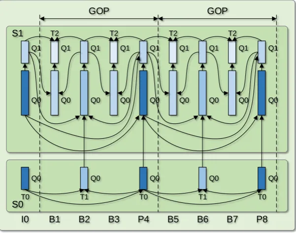
I B B P B B P B B P B B P
Fig. 1-2 I-, P- and B-frames in a Group of Pictures (GOP).
In most existing video coding standards, a video sequence comprises three types of
frame, as shown in Fig. 1-2.
1. I-frame (Intra-coded frame): I-frames are encoded without reference to any other
fra-mes, and contain only intra-coded macroblocks (these are blocks within an intra-coded
frame as described in subsection 2.2.1). From the perspective of compression, an
I-frame is the least efficient of the three types of I-frame.
2. P-frame (Predictive-coded frame): P-frames are encoded using the coding results of
previous I- and P-frames, and also used as a reference for the inter-frame coding of
subsequent frames. In the latest standards, macroblocks in P-frames are either
intra-coded or predictive-intra-coded.
previ-ous and subsequent frames and contain intra-coded, predictive-coded, and
bi-direct-ional-predictive-coded macroblocks. Generally, a B-frame requires the least number of
bits to encode, which makes it the most efficient of the three types of frame.
Encoder
Decoder
S˜ n
enʹ
Snʹ
Sn en enʹ
enʹ enʹ
S˜ n
Predictor
Entropy decoder
Quantiser
- Entropy
encoder
+
Predictor
Fig. 1-3 Block diagram of a typical predictive codec.
The basic principle of predictive coding is to use the previous samples to estimate the
value of the current sample. The residual or prediction error between the actual value and
the estimate then forms the signal to be further processed. It is obvious that, the more
accurate the prediction the lower is the resulting redundancy, and the more efficient the
coding process. The block diagram of a typical predictive codec is illustrated in Fig. 1-3;
notations are also introduced at appropriate points. In the diagram, the prediction ˜Sn of the current sampleSn is a linear combination of weighted previous samplesSi,i=1, ...,
n−1.
˜
Sn= n−1
X
i=1
αiSi (1.3)
Instead of directly coding the current sampleSn, the prediction erroren, which normally has less variance and energy than the original sampleSn, is coded.
Some quantisation noiseqn is added by the quantiser to the prediction error.
en0 =en+qn (1.5)
At the decoder, the inverse procedure is performed to restore the original sample. The
reconstructed prediction ˜Snis added toen0 to form the reconstructed output sampleSn0.
Sn0 =en0+S˜n=en+qn+S˜n=Sn+qn (1.6) Note that the difference between the original sample and the reconstructed sample at the
decoder is the quantisation noiseqn.
1.1.2 Transforms and Quantisation
Transform coding has proved to be an efficient tool to eliminate spatial redundancy in
im-ages or videos, therefore it forms an important component of almost all video coding
sys-tems[10]. Although different transformations are used in different video coding systems,
they all share the same function of mapping a group of pixel samples into a different
do-main. As the transformation does not generate any compression, it is generally followed by
quantisation and entropy coding. In the quantisation operation, the transform coefficient
is assigned one of a finite number of discrete values by rounding and truncation.
Conse-quently, the number of possible values of transform coefficients is reduced, thus resulting
in compression.
Transforms
The motivation for transforming a signal from the time domain to the frequency domain is
to acquire a more compact representation of the signal. Due to the prevalence of
homoge-nous content in natural images, the transform concentrates the most energy in the lower
frequency components, while the high frequency components have little energy. Since
discarded or reduced by applying a coarse quantisation to the higher frequency
compo-nents. When applying the above operations, compression is obtained, but a quantisation
error is necessarily introduced[11].
In a block-based coding scheme, each frame is divided into a number of blocks and
the blocks are transformed to another domain. Without loss of generality, the transform
process can be written asR=TSTt, whereSdenotes a block in the pixel domain,Rrefers
to the representation of the block in a specific transform domain,Tis a transform matrix
andTtis the transpose matrix ofT. From the perspectives of feasible implementation and
compaction efficiency, some of the transforms considered for image and video
compres-sion are the Discrete Fourier Transform (DFT), Discrete Hadamard Transform (DHT)[12],
Discrete Cosine Transform (DCT)[13], and Discrete Sine Transform (DST). Among these,
the DCT transform has become the common choice for most image and video coding
stan-dards.
For an 8×8 block of pixels, the Two-Dimensional (2D) DCT is expressed as
F(u,v) =1
4c(u)c(v) 7
X
x=0 7
X
y=0
f(x,y)cos
(2x+1)uπ
16
cos
(2y +1)vπ
16
(1.7)
where 0≤u≤7, 0≤v≤7 and
c(u),c(v) =
1 p
2 ifu,v=0
1 otherwise
(1.8)
In equation (1.7), f(x,y)denotes the intensity of a pixel sample at position(x,y)and
F(u,v)refers to the DCT transform coefficients. The transform coefficientF(0, 0) repre-sents the Direct Current (DC) value of the block and the remaining 63 transform
coeffi-cients are the Alternating Current (AC) coefficoeffi-cients. The inverse 2D DCT is thus defined
as
f(x,y) =1
4 7
X
u=0 7
X
v=0
c(u)c(v)F(u,v)cos
(2x+1)uπ
16
cos
(2y +1)vπ
16
(1.9)
The wide usage of the DCT is credited to the following benefits that it offers[14]: 1)
The DCT provides approximate compaction efficiency to the optimum Karhunen Loève
Transform (KLT) for images containing homogeneous content; 2) Due to the separability of
the 2D DCT, it can be implemented through a series of 1D DCTs in the horizontal direction,
followed by the vertical direction; 3) The DCT is independent of the image content; 4) Fast
DCT and Inverse DCT (IDCT) algorithms are widely available for efficient hardware and
software implementation.
(a) an original image in Bus sequence (b) an 8×8 block in pixel domain
(c) the 8×8 block in numerical form (d) the 8×8 block in the transform domain
164 169 169 164 161 148 155 166
162 169 167 164 166 155 157 162
163 165 167 165 162 157 161 163
170 171 171 168 167 167 167 162
170 171 173 173 172 170 169 163
169 168 169 171 168 163 165 161
162 162 165 166 162 153 159 161
163 167 167 163 163 160 169 165
1318 17 -3 -13 3 0 -6 6
-6 6 2 -6 3 -6 1 1
-18 -1 6 -9 3 -4 -2 2
4 5 -3 -1 4 0 0 -1
11 0 3 1 -4 0 0 0
-8 3 3 -4 3 1 0 0
2 -1 3 0 -1 2 0 -1
[image:29.595.132.493.279.657.2]-3 -2 -1 -2 1 0 1 -1
Fig. 1-4 An example of the forward DCT transform.
8×8 spatial block to a block of 8×8 frequency coefficients is presented in Fig. 1-4.
Fig. 1-4(a) is the 50thframe of the ‘Bus’ video test sequence; Fig. 1-4(b) shows the high-lighted 8×8 block of Fig. 1-4(a) in the pixel domain; the 8×8 block is represented in
nu-merical form in Fig. 1-4(c); Fig. 1-4(d) shows the transform coefficients of the 8×8 block
after application of the DCT. From Fig. 1-4(d), it can be seen that the values of the DCT
coefficients decrease as the horizontal and vertical frequencies increase. Most of the
en-ergy of the 8×8 block is concentrated towards the top-left corner corresponding to the low
horizontal and low vertical frequency regions.
Quantisation
The quantisation operation is usually performed after the transform, and is a necessary
procedure in lossy video compression. The transform coefficients are mapped to a finite
set of discrete amplitudes represented by a finite number of bits. The less important
trans-form coefficients, which do not have a significant influence on the picture quality, are
re-moved or eliminated. The more important transform coefficients are retained.
Specifi-cally, a coarse quantisation is performed on the high frequency components and a fine
quantisation on the low frequency components, since the HVS is more sensitive to the
uniform regions. Quantisation therefore leads to a significant reduction in the bit rate and
hence provides compression.
Quantisation rounds or truncates a transform coefficient to the nearest integer.
Gen-erally, this process is irreversible, as it is a many-to-one mapping.
A general quantisation process is described as
Q(u,v) =round
F(u,v)
Qs
(1.10)
whereQ(u,v)refers to the quantisation index,Qsis a quantisation step size, andround indicates the rounding function. The transform coefficient is reconstructed by rescaling
original value.
˜
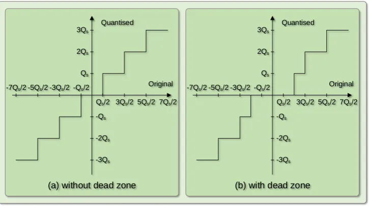
F(u,v) =Qs·Q(u,v) (1.11) where the ˜F(u,v)is the reconstructed transform coefficient. A uniform quantiser with a quantisation step sizeQs and an uniform quantiser with a ‘dead zone’ are illustrated in Fig. 1-5. In Fig. 1-5(b), the dead zone is an enlarged interval around zero, which is used
to reduce to zero more small transform coefficients. The quantisation results of the DCT
coefficients in Fig. 1-4(d) using the uniform quantiser without dead zone and the quantiser
with dead zone are illustrated in Fig. 1-6.
Quantised
Original Quantised
(a) without dead zone (b) with dead zone
-Qs/2
-3Qs/2
-5Qs/2
5Qs/2
3Qs/2
Qs/2
Qs
2Qs
3Qs
-3Qs
-2Qs
-Qs
7Qs/2
-7Qs/2
-Qs/2
-3Qs/2
-5Qs/2
5Qs/2
3Qs/2
Qs/2 7Qs/2
-7Qs/2 Original
Qs
2Qs
3Qs
-3Qs
-2Qs
[image:31.595.133.496.312.515.2]-Qs
Fig. 1-5 Uniform quantisers.
1.1.3 Entropy Coding
Entropy coding is used to achieve further compression by reducing the statistical
redun-dancy within the quantised coefficients or symbols. Relatively shorter codewords are
as-signed to the symbols that occur more frequently, and vice versa. The entropy coder
at-tempts to minimise the average number of bits per symbol that are required to represent
commonly used in image and video compression standards.
165 2 0 -2 0 -1 1
0 0 0 0 0 0 0
1 0 -1 0 -1 0
-2
1
1
-1
0
0 0 0 0 0 0 0
-1
0 1 -1 0 -1 0
1 0 0 1 0 0
0 0 0 -1 0 0
0 0 -1 0 0
0 0 0 0 0 0
0
(a) uniform quantiser without dead zone (b) uniform quantiser with dead zone
0
165 2 0 -2 0 0 0
0 0 0 0 0 0 0
0 0 0 0 0 0
-2
0
1
-1
0
0 0 0 0 0 0 0
0
0 0 -1 0 0 0
0 0 0 0 0 0
0 0 0 0 0 0
0 0 0 0 0
0 0 0 0 0 0
0
0
Fig. 1-6 Quantisation results with quantisation step sizeQs=8.
Many blocks contain a few significant non-zero coefficients and a large number of
zero coefficients after transformation and quantisation, as shown in Fig. 1-6. These sparse
blocks are normally coded by the following steps.
1. Reorder the quantised coefficients
For a natural image, the non-zero transform coefficients are concentrated close to the
top-left DC coefficient, and the magnitude of the transform coefficients decreases
rapi-dly along the horizontal and vertical directions towards the bottom-right. The
trans-form coefficients are therefore required to be reordered in a more compact
represen-tation. The optimum scan manner would be to reorder the coefficients in descending
order of their magnitude, thus resulting in a series of zeros at the end of the reordered
sequence. In practice, scanning in a zig-zag manner performs well, efficiently
group-ing the zero and non-zero coefficients. As shown in Fig. 1-7, the zig-zag scan of the
transform coefficients commences at the top-left corner of the 8×8 transform
coeffi-cient matrix, where the lower frequency components reside, to the higher frequency
2. Run Length Coding (RLC)
As the result of the zig-zag scan order operation, a 1D array is produced in which most
non-zero coefficients are encountered before the zero coefficients. Instead of coding
each coefficient individually, so called Run Length Coding (RLC) is employed to reduce
the redundancy within the series of coefficients. The codewords of RLC comprise a
series of (run, level) pairs, where ‘run’ represents the number of zero coefficients that
precede a non-zero coefficient and ‘level’ refers to the value of the non-zero coefficient.
An End-of-Block (EOB) symbol is used to indicate that all remaining coefficients are
zero.
165 2 0 -2 0 -1 1
0 0 0 0 0 0 0
1 0 -1 0 -1 0
-2
1
1
-1
0
0 0 0 0 0 0 0
-1
0 1 -1 0 -1 0
1 0 0 1 0 0
0 0 0 -1 0 0
0 0 -1 0 0
0 0 0 0 0 0
0
(a) uniform quantiser without dead zone (b) uniform quantiser with dead zone
0
165 2 0 -2 0 0 0
0 0 0 0 0 0 0
0 0 0 0 0 0
-2
0
1
-1
0
0 0 0 0 0 0 0
0
0 0 -1 0 0 0
0 0 0 0 0 0
0 0 0 0 0 0
0 0 0 0 0
0 0 0 0 0 0
0
0
Fig. 1-7 Zig-zag scan of quantisation coefficients.
Consider the zig-zag ordered coefficients derived in Fig. 1-7(b),
165, 2, 0, -2, 0, 0, -2, 0, 0, 0, 1, 0, 0, 0, 0, 0, 0, -1, 0, 0, -1, 0,
0, 0, 0, 0, 0, 0, 0, 0, 0, 0, 0, 0, 0, 0, 0, 0, 0, 0, 0, 0, 0, 0,
0, 0, 0, 0, 0, 0, 0, 0, 0, 0, 0, 0, 0, 0, 0, 0, 0, 0, 0, 0.
RLC converts the coefficients into the following (run, level) pairs,
3. Variable Length Coding (VLC)
A variable length entropy coding algorithm, such as Huffman coding[15]or arithmetic
coding[16], is employed to encode the (run, level) data into a set of compact binary
bitstreams. The entropy coder assigns a shorter codeword to a (run, level) pair with
high probability of occurrence and a longer codeword to an infrequently occurring pair,
so that the average bit rate is minimised.
1.2
International Video Coding Standards
The standardisation of video coding algorithms has greatly stimulated the development of
video compression technology. This has enabled a variety of new visual applications in the
fields of communication, multimedia, and broadcasting[17]. Video coding
standardisa-tion work has been conducted since the early 1980s, and a series of video coding standards
have been developed, each targeted at different application scenarios. The Video Coding
Experts Group (VCEG) in the International Telecommunications Union
Telecommunica-tion StandardisaTelecommunica-tion Sector (ITU-T), the Moving Picture Experts Group (MPEG) in the
In-ternational Standards Organisation (ISO) and InIn-ternational Electrotechnical Commission
(IEC), and a combination of the two known as the Joint Video Team (JVT) are the major
organisations in the development of the standards. The evolution of video compression
standards over the last three decades is summarised in Fig. 1-8.
1992 1994
1990 1996 1998 2000 2002 2004 2006 2008 2010 2012 2014 2016 H.263 H.263+
H.261
H.262/MPEG-2 H.264/MPEG-4 AVC H.265/MPEG-H HEVC
MPEG-1 MPEG-4Visual H.263++ ITU-T
standards
Joint standards
MPEG standards
1.2.1 ITU-T H.261 and H.263
Generally, the ITU-T contributes work for real-time telecommunication applications, such
as the H.261 standard[18]for transmission over Integrated Services Digital Network (ISDN)
lines and the H.263 standard[19]for very low bit rate communications over Public Switched
Telephone Network (PSTN) channels. The H.261 and H.263 standards are designed to offer
high compression ratios for full colour video transmission with very low delay.
H.261
The ITU-T H.261 standard was developed for video telephony, video conferencing and
other audiovisual services over ISDN channels at bit rates ofn×64 kbits/s, wherenis an integer with values between 1 and 30. H.261 was the first video coding framework that was
widely used in practical terms. It adopted a hybrid DCT/Differential Pulse-Code
Modula-tion (DPCM) coding scheme with integer pixel moModula-tion compensaModula-tion. Two frame formats
are supported in H.261: Common Intermediate Format (CIF) and Quarter Common
In-termediate Format (QCIF) using a 4:2:0 chroma sampling scheme, i.e. the resolution of
the luminance component is 352×288 for CIF and 176×144 for QCIF and the horizontal
and vertical chrominance resolutions are half those of the luminance component. The
concept of a macroblock was originally suggested in H.261, where a macroblock is a basic
processing unit comprising 16×16 pixels. H.261 elaborated the video coding techniques
of prediction with motion compensation, DCT transform coding, quantisation, VLC and
rate control.
A block diagram of an H.261 encoder is illustrated in Fig. 1-9. Inter-frame prediction is
used to remove the temporal redundancy and transform coding is used to remove the
spa-tial redundancy. As H.261 is designed to operate in real-time video telephony and video
conferencing applications, motion compensation is optional and only forward motion
es-timation is allowed. H.261 was a successful video coding standard and was regarded as a
meth-ods in H.261 were adopted for future video coding standards, and H.261 was the first
ex-ample of a transform-based video coder.
DCT
IDCT Dequantiser Quantiser
Coding controller
Entropy
encoder Buffer
Motion compensation
Frame memory
Motion estimation Loop
filter
+
-Video input
Bitstream
Fig. 1-9 Block diagram of a typical H.261 video encoder.
H.263
The ITU-T H.263 video coding standard was developed to support low delay video
tele-phony applications over PSTN networks at bit rates of less than 64 kbits/s. The original
version of H.263 was approved as a standard in early 1996; afterwards some new features
and improvements were introduced (also known as H.263+and H.263++) in 1998 and 1999
respectively.
The coding structure of H.263 is inherited from H.261, but more optional modes and
even more frame formats, from SQCIF (128×96 pixels) to 16CIF (1408×1152 pixels), are
supported. These new features allow H.263 to be applied in various application scenarios
and transmission circumstances.
The following improved features enable H.263 to offer obvious superiority over H.261.
1. Half pixel precision motion compensation: In the H.261 codec, only integer pixel
pre-cision motion estimation and compensation were defined, whereas in H.263 half pixel
precision was used to achieve better motion compensation. The prediction accuracy is
2. Three-Dimensional (3D) VLC: The VLC codeword in H.263 was extended to a 3D
for-mat of (last, run, level). Similar to the codeword in H.261, ‘run’ indicates a run length
of zero coefficients that precede a non-zero coefficient and ‘level’ refers to the value of
the non-zero coefficient. The EOB element of H.261 is replaced by a new element ‘last’,
which is a binary variable. ‘0’ means that there are more non-zero coefficients in the
block, and 1 means that this is the last non-zero coefficient in the block.
3. Improved MV coding: The MVs of the three neighbouring macroblocks are used to
pre-dict the MV of the current macroblock. Instead of directly encoding the MV, the
predic-tion error is encoded using VLC.
By applying the above techniques, compared to H.261, H.263 achieves 50% or more
savings in the bit rate needed to represent video at a given perceptual quality at very low
bit rates. In terms of Signal-to-Noise Ratio (SNR), H.263 can provide about 3dB gain over
H.261 at these very low bit rates.
1.2.2 ISO/IEC MPEG-1, MPEG-2, and MPEG-4 Visual
MPEG, formally, Working Group 11 (WG11) of ISO/IEC Joint Technical Committee 1 (JTC1)/
SubCommittee 29 (SC29) was formed to set standards for audio and video compression
[20, 21]. The most notable MPEG standards to date are MPEG-1[22, 23]for audiovisual
data storage on CD-ROM, MPEG-2[24–26]for high quality moving picture applications
and MPEG-4 Visual[27]for the coding of audiovisual objects.
MPEG-1
MPEG-1 was the first MPEG standard and targeted at the storage of moving pictures and
audio on hard disks at the bit rate of 1.5 Mbits/s to 2 Mbits/s. It accommodates
progres-sive scan video and operates on Source Input Format (SIF) video (352×240, 352×288, or
320×240 pixels) at 25 fps and 29.97 fps. In fact, MPEG-1 is built on the work of the Joint
many of coding techniques used in the JPEG and H.261 standards. Both MPEG-1 and
H.261 adopted the hybrid DCT/DPCM codec scheme. However, the following features
de-fined in MPEG-1 distinguish it from H.261.
1. Types of frame: Only forward prediction is allowed in H.261, while in MPEG-1 a so
called B-frame is defined which is predicted from frames in both the forward and
back-ward directions. Furthermore, a unique frame type is used in MPEG-1 to facilitate
fast forward and backward preview, namely D-frame, which is encoded using only DC
transform coefficients.
2. Accuracy of motion estimation: Half pixel precision is used for motion estimation
in MPEG-1, while H.261 restricts the motion estimation to integer pixel accuracy.
Al-though the half pixel precision increases the computational complexity of the codec, a
better coding efficiency is gained.
3. Motion search range: H.261 is used mainly for video telephony and video
conferenc-ing, where the motion activity is simple and slow. Unlike H.261, MPEG-1 is normally
used for the coding of movies, which contain larger movement and more complex
ac-tivity. Consequently, a larger MV search range is supported in MPEG-1.
MPEG-2
The MPEG-2 standardisation activity was started in 1991 and targeted at high quality video
coding at bit rates of 4-15 Mbits/s for Video on Demand (VOD), digital broadcast
televi-sion, and digital storage media such as DVD. Three years later in 1994, MPEG-2 was
ap-proved by ISO/IEC as an international video coding standard. This standard was also
rec-ommended by the ITU-T as H.262. MPEG-2 was developed from MPEG-1 but included
some advanced features to accommodate video applications of higher picture quality,
in-terlaced coding, and a more flexible syntax. MPEG-2 achieved tremendous commercial
success and was employed in digital terrestrial TV broadcasting, digital cable TV, and many
The basic coding structure of MPEG-2 is the same as that of MPEG-1, but the following
enhancements enable MPEG-2 to show substantial superiority over MPEG-1 and H.261.
1. Supported source format: MPEG-2 supports a set of larger frame sizes ranging from
CIF (352×288 pixels) to HDTV (1920×1080 pixels). Both progressive and interlaced
scan coding are supported in MPEG-2, while MPEG-1 was designed only for progressive
video coding.
2. Scalability function: The scalability modes of MPEG-2 enable interoperability among
different services or accommodation of different receivers and networks upon which a
single service may operate. MPEG-2 allows the decoder to decode a subset of the full
bitstream in order to display a video sequence at a reduced quality, spatial or temporal
resolution.
3. Alternate scan order: As well as the zig-zag scan order of DCT coefficients used in
MPEG-1 and H.261, MPEG-2 has an alternate scan order to accommodate interlaced
video.
4. Quantisation of DCT coefficients: Both linear and non-linear quantisation of DCT
co-efficients are supported in MPEG-2[29, 30]. The non-linear quantisation increases the
precision of quantisation at high bit rates by employing lower quantiser scale values.
This improves picture quality in low contrast areas.
MPEG-4
There are two video coding standards defined in MPEG-4: MPEG-4 part 2 (also known as
MPEG-4 Visual) and MPEG-4 part 10 (also known as MPEG-4 AVC)[27, 31, 32]. In contrast
to conventional block-based video coding standards, MPEG-4 Visual was the first
object-based visual compression scheme which enables not only efficient compression, but also
enhanced flexibility, extensibility and accessibility for a wide range of applications. In the
object-based MPEG-4 video coding system, each video scene is made up of a number of
shape, motion and texture. Each VOP is encoded independently to others using a coding
algorithm similar to H.263 and context-based arithmetic coding is employed to code the
shape of the VOP. In this way, MPEG-4 achieves the following primary features.
1. Higher compression efficiency: A number of advanced coding tools are used to
in-crease the coding efficiency of MPEG-4 including: DC prediction, AC prediction,
alter-nate scan order, and global motion compensation.
2. Interactive functionality: A video scene can be coded as a set of VOPs rather than a
series of frames. This is a novel feature in MPEG-4 and allows both foreground and
background to be coded independently. This feature enables the user to access and
manipulate individual objects in a video scene.
3. Universal access functionality: Several mechanisms were incorporated into
MPEG-4 to handle transmission errors and maintain successful video transmission in
error-prone network environments. MPEG-4 also supports spatial and temporal scalability,
which provide flexible solutions over a wide range of transmission bit rates.
1.2.3 ITU-T H.264/MPEG-4 AVC
The video coding experts from ITU-T VCEG and ISO/IEC MPEG formed the JVT in 2001.
The collaborative result, H.264 or MPEG-4 part 10 Advanced Video Coding (AVC) was
fi-nalised in March 2003[32–37]. This standard aimed to achieve a coding efficiency at least
twice better than that of the earlier video codecs, such as H.263 or MPEG-4 Visual.
H.264/MPEG-4 AVC has been used for many applications: broadcasting HDTV over
cable, terrestrial and satellite channel video transmission, storage of high quality video on
optical and magnetic storage devices, and some other emerging video applications such
as VOD, Internet Protocol Television (IPTV) and mobile video communications.
H.264/MPEG-4 AVC introduced a number of new features that provide better coding
efficiency than its predecessors. Some of the notable features are as follows:
increased up to 16 in a more flexible fashion than that of earlier standards.
2. Variable block size motion compensation: The block sizes used in H.264/MPEG-4 AVC
range from 4×4 to 16×16 pixels.
3. Quarter pixel precision for motion compensation
4. Weighted prediction
5. Directional spatial prediction for intra-coding
6. Exact match transform
7. Hierarchical block transform
8. In-loop deblocking filtering
9. Decoupling of referencing order from display order.
The above and some other techniques enable H.264/MPEG-4 AVC to achieve a
signif-icant improvement over earlier standards under a wide range of circumstances.
1.2.4 ITU-T H.265/MPEG-H HEVC
H.265/MPEG-H High Efficiency Video Coding (HEVC) is the most recent joint
standard-isation work of the Joint Collaborative Team on Video Coding (JCT-VC), which is formed
from the ITU-T VCEG and the ISO/IEC MPEG standardisation bodies[38].
The first version of the H.265/MPEG-H HEVC standard[39]was published in January
2013, and further improvements are still under development. A scalable extension and
multi-view extension of H.265/MPEG-H HEVC are being developed and will be finalised
in the near future. In order to satisfy new challenges posed by emerging video
applica-tions such as Ultra High Definition Television (UHDTV) and Three-Dimensional
Televi-sion (3DTV), HEVC aims to further reduce the bit rate by a further 50% compared to the
current state-of-the-art H.264/MPEG-4 AVC standard[40]. H.265/MPEG-H HEVC features
a comprehensive suite of coding tools enabling a significant improvement over the prior
standards. The new features of H.265/MPEG-H HEVC along with those of H.264/MPEG-4
T able 1-1 C ompar ison of tools in H.264 / MP EG-4 A V C and H.265 / MP EG-H HE V C ∗ F eatur es H.264 / A V C HE V C P ar titioning C oding P ar titioning 16 × 16 macr oblock V ar iable , lar ge siz e P rediction P ar titioning Q uadtr ee-based str uctur e Irr egular , lar ge siz e T ransfor m P ar titioning 4 × 4 and 8 × 8 R ectangular , lar ge siz e M otion MVP D er iv ation M edian MV competition M otion S har ing N o Y es M otion Infer ence B _DIRECT , SKIP P_DIRECT ; E nhanced B_DIRECT ; SKIP; T emplate matching
Inter Prediction
[image:42.595.184.461.124.718.2]1.3
Research Contributions
The main contributions detailed in this thesis relate to improved algorithms for techniques
employed in the scalable extension of H.264/AVC standard.
The mode selection process in SVC requires a much larger amount of computation
than the scalable profiles of previous video coding standards, as SVC intends to support
temporal, spatial and quality scalability. Furthermore, SVC demonstrates significantly
im-proved coding efficiency compared with existing video coding standards. However, this is
achieved at the cost of additional computation. This thesis describes methods to reduce
the computational complexity of the SVC encoder without significantly degrading the Rate
Distortion (RD) performance. Chapter 4 presents a simple and efficient mode selection
algorithm and this process is extended into a hierarchical scheme in chapter 5. The
pro-posed fast mode selection algorithm makes full use of inter-layer, temporal and spatial
correlation, as well as the texture information of each macroblock. It produces
state-of-the-art performance in terms of encoding time reduction.
An inter-layer prediction mechanism to reuse the coded lower layer data for encoding
the corresponding enhancement layer is employed in SVC. However, the effects of
inter-layer prediction are not taken into consideration in the rate control scheme of SVC. The
ex-isting RD models cannot accurately represent the RD properties of the prediction modes.
Chapter 6 analyses the RD statistical properties of the different prediction modes and
de-velops a more accurate RD model for the spatial enhancement layers. Furthermore, some
encoding results of the base layer can be used to inform the encoding of the
enhance-ment layers, thus benefiting from the bottom-up coding structure of SVC. An optimised
Mean Absolute Difference (MAD) prediction model for the spatial enhancement layers is
detailed. Simulation results show that the proposed methods achieve better rate control
accuracy than the default rate control scheme of SVC, Furthermore, the proposed
1.4
Thesis Outline
This chapter provided a brief review of fundamental techniques in video coding,
includ-ing predictive codinclud-ing, transform codinclud-ing, quantisation and entropy codinclud-ing. Buildinclud-ing on
the video compression principles mentioned above, currently used and evolving
interna-tional video coding standards: H.261, MPEG-1, H.262/MPEG-2, H.263, MPEG-4 Visual,
H.264/MPEG-4 AVC, and H.265/MPEG-H HEVC, are briefly described. This background
knowledge is important to further discussions in this thesis.
The next chapter discusses the importance and advantages of scalable coding in video
communication and also describes the basic principles of the scalable extension of the
H.264/AVC standard (SVC). Chapters 3 through to 6 describe my main contributions to the
field. These include performance analysis of advanced scalable video codecs (chapter 3)
and improvements made to techniques employed in the SVC standard (chapters 4, 5, and
6). Finally, concluding remarks and suggestions for future work are included in chapter 7.
The following provides a detailed outline of each chapter.
† Chapter 2 reviews the functional structure of SVC. The basic concept of scalability types
as well as the advanced techniques incorporated in SVC are then explained to provide
the prerequisite knowledge required for the remaining chapters. Two problems to be
addressed in this thesis are also presented.
† Chapter 3 provides an analytic comparison of the three advanced scalable video coding
schemes, SVC, Motion JPEG2000, and Wavelet Scalable Video Coding (WSVC). Coding
efficiency in terms of RD performance is examined in detail.
† Chapter 4 initially reveals the relationship between best coding mode and motion
ac-tivity, then presents a fast inter-frame and inter-layer mode selection algorithm
utilis-ing the motion activity in the video sequence.
† Chapter 5 proposes a hierarchical fast mode decision scheme that exploits the
performance comparison with state-of-the-art algorithms is presented.
† Chapter 6 presents a novel rate control algorithm for the enhancement layers of SVC, in
which a new RD model and an optimised MAD prediction model are described. With
the proposed rate control algorithm, good bit rate control and a higher coding
effi-ciency is achieved.
† Chapter 7 summarises the thesis, conclusions are drawn, and some directions for
Scalable Video Coding
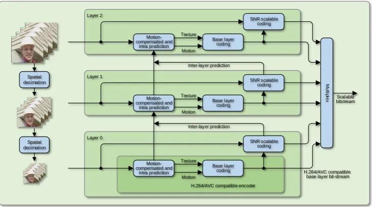
This chapter reviews the scalable extension of the H.264/AVC standard by describing its
functional structure, basic modes of scalability and some associated techniques. In
or-der to generate a scalable video bitstream, a layer-based coding scheme is employed. A
H.264/AVC compatible encoder is used for the Base Layer (BL) and a scalable video
en-coder for the Enhancement Layers (ELs). In each layer, motion-compensated prediction
and intra-prediction are employed as for single layer coding. Furthermore, when encoding
the enhancement layers, the inter-layer prediction mechanisms are introduced to remove
the redundancy between layers. SVC mainly supports three kinds of scalability, in
tem-poral frame rate, spatial resolution, and reconstruction quality. In the next section, the
layer-based coding scheme and the three basic types of scalability are described in detail.
In section 2.2, SVC is discussed in terms of its prediction, transform, quantisation, and
en-tropy coding tools. Sections 2.3 and 2.4 highlight two problems which the work presented
2.1
Overview of the Scalable Extension of H.264
/
AVC
Early video coding systems encoded video at a fixed target bit rate for a specific
applica-tion. An increasing number of applications imposed higher demands on the nature of the
video service provided. High coding efficiency is not the only goal, but also the ability to
meet various client terminal capabilities, network conditions, and user demands. In order
to meet the requirements of these new video coding challenges, encoded video that
sup-ports a highly scalable, easily adaptable, and fully accessible bitstream has attracted much
attention in both industry and academia[42,43]. The simulcast technique provides a
sim-ple solution for scalable video. It independently encodes multisim-ple versions of the video at
different resolutions and transmits that version which is most appropriate for the
band-width available. Due to the low efficiency of simulcast, a better solution that guarantees
ef-ficient data transmission to video clients with diverse needs over heterogeneous networks
is desirable[44]. As shown in Fig. 2-1, scalable video coding aims to encode the original
video once, but permits the compressed bitstream to be decoded with a lower frame rate,
smaller spatial size or degraded quality in accordance with the device capabilities,
net-work characteristics and user requirements. Temporal, spatial and quality scalability can
be achieved by selectively transmitting and decoding the required substreams. Compared
with simulcast, scalable video coding possesses a greater ability to satisfy various needs
and to achieve higher coding efficiency. The challenges presented have meant that
scal-able video coding has become an active research topic, attracting extensive attention from
experts in the field of video processing.
The JVT of ITU-T VCEG and ISO/IEC MPEG has defined a scalable extension to the
H.264/AVC standard, namely SVC. SVC incorporates the many new coding tools which
are employed in H.264/AVC to improve coding efficiency and robustness. These
tech-niques include: 1) Variable size block matching for motion estimation and compensation,

![Fig. 2-7 Nine prediction patterns of intra 4×4 type (taken from [30]).](https://thumb-us.123doks.com/thumbv2/123dok_us/9608391.463808/59.595.131.498.395.650/fig-prediction-patterns-intra-type-taken.webp)