University of Warwick institutional repository: http://go.warwick.ac.uk/wrap
A Thesis Submitted for the Degree of PhD at the University of Warwick
http://go.warwick.ac.uk/wrap/56925
This thesis is made available online and is protected by original copyright. Please scroll down to view the document itself.
Developments of New Techniques
for Studies of Coupled Diffusional and Interfacial
Physicochemical Processes
By
Tahani Mohammad Bawazeer
A thesis submitted for the degree of
Doctor of Philosophy
Department of Chemistry
United Kingdom
For
my parents…
my husband…
and my Children…
I would never have
reached this point without you,
ii
Table of Contents ii
List of Illustrations v
List of Tables xii
List of Abbreviations xiii
List of Symbols xv
Acknowledgment xvii
Declaration xviii
Abstract xix
Chapter 1 Introduction 1
1.1 Fluorescence Confocal Laser Scanning Microscopy (CLSM) 1
1.1.1 Literature Survey 1
1.1.2 CLSM Principle 4
1.1.3 Fluorescence 6
1.1.3.1 Fluorescein 8
1.2 Electrochemistry and Microelectrodes 11
1.2.1 Introduction to electrochemistry 11
1.2.2 Dynamic electrochemistry 12
1.2.3. Mass transport 15
1.2.3.1 Diffusion 16
1.2.3.2 Convection 18
1.2.3.3 Migration 18
1.2.4 Ultramicroelectrodes (UME) 19
1.2.5 Linear Sweep Voltammetry and Cyclic Voltammetry 22 1.2.6 Scanning electrochemical microscopy (SECM) 25
1.2.6.1 Negative Feedback 26
1.2.6.2 Positive Feedback 28
1.4 Finite Element Modelling (FEM) 28
1.5 Aims of the Thesis 31
1.6 References 33
Chapter 2 Experimental Methods 37
iii 2.2 Device Microfabrication and Characterisation 39
2.2.1 Pt Ultramicroelectrode (UME) Fabrication and Characterisation 39 2.2.2 Optical Transparent Single-Walled Carbone Nanotubes
Ultramicroelectrodes (OT-SWNTs-UMEs) mat Fabrication
42
2.3 CLSM Experiments 47
2.3.1 Visualisation of Electrochemical Processes at OT-SWNTs-UMEs 48 2.3.2 Visualization of Proton Diffusion at active and Modified Surfaces 51
2.4 Additional Instrumentation 58
2.4.1 Inductively Coupled Plasma Mass Spectroscopy (ICP-MS) 58 2.4.2 Fluoride Ion Selective Electrode (FISE) Studies 59
2.5 Finite Element Modelling 59
2.6 Solution Preparation 59
2.7 References 61
Chapter 3 Visualisation of Electrochemical Processes at Optically
Transparent Single-Walled Carbon Nanotubes
Ultramicroelectrodes (OT-SWNTs-UMEs)
62
3.1 Overview 62
3.2 Introduction to Carbone Nanotube 69
3.2.1 Characterisation of SWNTs ultrathin films 73 3.2.2 Characterisation of SWNTs disc OT-UMEs 74 3.3 Visualisation of the ORR at SWNTs disc OT- UME 76
3.3.1 Dynamic Visualisation of Ru(bpy)32+ concentration during CV measurements at SWNTs disc OT- UME.
79
3.3.2 Three dimensional concentration profiles of Ru(bpy)32+at the steady-state current.
81
3.4 Conclusion 85
3.5 References 87
Chapter 4 Transient Interfacial Kinetics, from Confocal Fluorescence
Visualisation: Application to Proton Attack the Treated
Enamel Substrate
90
iv
4.1.1 Enamel Structure 92
4.1.2 Enamel Dissolution 93
4.1.3 Enamel Dissolution Inhibitors 94
4.2 Proton Distribution at Disc UME 95
4.3 CLSM Visualisation of Proton Flux during Enamel Dissolution 96 4.3.1 Experimental Results and Analysis 97
4.4 Finite Element Model 103
4.4.1 Diffusion Coefficients 107
4.4.2 Insights from Simulations 109
4.5 Amount of Zinc and Fluoride Uptake on Treated Enamel 113
4.6 Conclusions 114
4.7 References 116
Chapter 5 Combined Confocal Laser Scanning Microscopy -
Electrochemical Techniques for the Investigation of Lateral
Diffusion of Protons at Surfaces
119
5.1 Biological Membranes 119
5.2 Supported Lipid Bilayer (SLB) Synthesis and Characterisation 123 5.3 Modification of Surfaces by Ultrathin Films 126
5.4 Proton Lateral Diffusion 128
5.5 Result and Discussion 132
5.5.1 Characterisation of SLB-Modified Surfaces by AFM 132 5.5.2 Measurement of proton diffusion at modified surfaces 134
5.6 Conclusion 145
5.7 References 147
Chapter 6 Conclusion 151
v
List of Illustrations
Chapter 1 Introduction 1
Figure 1.1 (a) Full-field illumination (b) Single point illumination 4
Figure 1.2 Schematic diagram of a confocal microscope 5 Figure 1.3 Schematic of 3D z-stack imaging in CLSM 6 Figure 1.4 A Jablonski diagram showing the origin of fluorescence, with the
photoexitation of an electron from (1) to (2) and emission light when the electron moves from (3) to (1)
7
Figure 1.5 Definition of Stokes shift 8
Figure 1.6 Illustration of pH vs. intensity of fluorescence after fluorescein excitation at 488 nm and detection at 530 nm
9
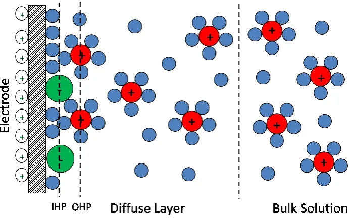
Figure 1.7 Molecular structures of neutral fluorescein and its anions 10 Figure 1.8 A diagrammatic representation of the electrical double layer
where the red cations are solvated with small blue circles representing water molecules, and large green anions are specifically adsorbed onto the electrode surface
12
Figure 1.9 The effect of the applied potential on the Fermi level 13 Figure 1.10 A schematic representation of a typical electrode reaction 14 Figure 1.11 Different geometries of electrodes and their diffusion fields: (a)
Disk electrode (b) Cylinder electrode and (c) Ring electrode Reproduced from reference
20
Figure 1.12 (a) Schematic of planar diffusion profile exhibited by a macroelectrode and (b) the hemispherical diffusion at disc UME
21
Figure 1.13 Showing the RG of an UME where rs is the radius of the whole UME and a is the radius of the metal wire
22
Figure 1.14 Typical CV responses for (a) a macroelectrode and (b) an ultramicroelectrode
23
Figure 1.15 (a) Schematic of negative feedback, for an UME near an insulating substrate and (b) Theoretical approach curve for a 25 µm diameter UME with an RG of 10, depicting negative feedback
27
Figure 1.16 (a) Schematic of positive feedback near a conducting substrate (b) Theoretical approach curve for a 25 µm diameter UME displaying positive feedback
vi Figure 1.17 (a) An example of a simple triangular mesh used for FEM and
(b)the same domain where the mesh is finer at two edges
30
Chapter 2 Experimental Methods 37
Figure 2.1 Conventional light microscope image of the tip of a 25 μm diameter platinum disc UME (a) from the side (b) the electrode surface
40
Figure 2.2 Cyclic voltammogram for the oxidation of 1 mM FcTMA at a 25-μm diameter Pt UME. The scan rate was 10 mV s-1
41
Figure 2.3 SECM experimental approach curve (red line) and the theory (blue line) towards inert glass substrate performed in 0.1 M KNO3
42
Figure 2.4 Schematic illustration the procedure for growing carbon nanotube ultrathin mats using catalysed chemical vapour deposition technique
43
Figure 2.5 (a) Schematic of the procedure used for fabricating SWNTs network disk UMEs, (bi) Geometry of the shadow mask used for microfabrication of Cr/Au bands for disk UME experiments, (bii) Photographs of SWNTs devices used in electrochemical experiments
45
Figure 2.6 Micro-Raman spectrum of SWNTs ultrathin mats grown on single crystal quartz
47
Figure 2.7 Schematic representation of the experimental setup used for visualising OT-SWNTs-UMEs
49
Figure 2.8 Schematic diagram of the clamp system developed for use with the confocal microscope
51
Figure 2.9 (a) Rise time for a current of 20 nA using homemade galvanostat and (b) corresponding change of the potectial applied to the UME working electrode
52
Figure 2.10 Describes the CLSM-SECM set-up where: (a) is a schematic detailing the components seen in (b); (b) is a photograph showing the UME and enamel sample inserted in the cell and immersed in solution
vii Figure 2.11 Experimental set up for SECM tip positioning and CLSM
experiments
55
Figure 2.12 Schematic (not to scale) of experimental arrangement for studies of proton diffusion at a SLB
57
Figure 2.13 Schematic of experimental arrangement for studies of proton diffusion in a thin layer
58
Chapter 3 Visualisation of Electrochemical Processes at Optically
Transparent Single-Walled Carbon Nanotubes
Ultramicroelectrodes (OT-SWNTs-UMEs)
62
Figure 3.1 a) AFM (3 nm × 3 nm) AFM images (full height scale=5 nm) of a SiO2 surface after cCVD growth of SWNTs. b) associated FE-SEM image of a SWNT network. The scale bar represents 5 μm. Taken from reference
71
Figure 3.2 (a) 1 µm × 1 µm tapping mode AFM height images of SWNT networks and ultrathin mats grown on single crystal ST-cut quartz substrate, using Co as the catalyst, sputter-deposited on the substrate 20 s prior to growth. (b) Micro-Raman spectrum of SWNT ultrathin mats grown on single crystal quartz
74
Figure 3.3 UV-Vis spectra of: blank cut quartz; SWNT mat grown on ST-cut quartz substrate; and ST-ST-cut quartz coated with S1818 positive photoresist
75
Figure 3.4 (a) Brightfield mode (b) and fluorescence mode images of an optically transparent carbon nanotube ultramicroelectrode (zoomed out and zoomed in). The images were recorded in the x-y
plane parallel to the electrode
76
Figure 3.5 CV of ORR and simultaneous change of solution light intensity as a function of potential, at a SWNT disc OT-UME (scan rate 10 mVs-1) for 0.1 M NaCl aqueous solution with 8 µM fluorescein and an initial pH 5. The arrows indicate the initial scan direction. The intensity values were collected from the middle of the UME surface, from a 35 µm diameters region of interest (ROI). The fluorescence mode insets illustrate the development of pH
viii gradients as a function of potential. The scale bars are 250 µm
Figure 3.6 (a) Fluorescence intensity at a potential of -1.0 V in 0.1 M NaCl solution with 8 µM fluorescein in the xy, xz and yz planes. The scale bar in the xy image is 250 µm. The red and white lines in xz
and yz cross sections indicate the photoresist and OT UME surface. (b) A graph of intensity below (B) and above (A) the OT-UME plane in 35 µm diameter ROI. The dashed line indicates the electrode surface
78
Figure 3.7 (a) CV (red) and simultaneous change of the fluorescence intensity (black: scan rate 5 mV/s) for the oxidation of 10 mM Ru(bpy)32+ in aqueous solution in 0.1 M NaCl. The arrows indicate the forward scan direction. The intensity values were collected from the 35 mm diameter region of interest at the centre of the UME. Intensity values and current values were normalised by the initial intensity value at time = 0 s (It=0) and the steady-state limiting current value (ilim), respectively. The insets show fluorescence profiles near the OT-CNT-UME surface during Ru(bpy)32+ oxidation. The scale bars are 25 mm. (b) Relationship between normalised current and fluorescence intensity change for forward andreverse scan directions in the range of quartile potentials of the voltammetric signature
80
Figure 3.8 The change of solution intensity over time during stepping up the potential from 0 V to the potential of the mass transport limiting current (1.2 V), determined from the CV for 10 mM Ru(bpy)32+ aqueous solution in 0.1 M NaCl. The inlets indicate the formation of the diffusion zone at the UME surface. The scale bar is 25 µm
82
Figure 3.9 Cross sectional light intensity change below and above the UME surface before (left) and after (right) the potential step for the 1 mM (a), 5 mM (c), and 10 mM (e) Ru(bpy)32+ in 0.1 M NaCl (e). All images were collected with the z-volume 150 µm (vertical white dashed line) and the z-step 2 µm. Z-stack before the potential step and during the steady state for the 1 mM (b), 5 mM (d), and 10 mM (f) Ru(bpy)32+ in 0.1 M NaCl. The scale bars in (a,
ix c) and (e) are 25 µm. Dark blue arrows indicate the -position of the electrode surface in both scans. The light intensity values were normalised taking into account the intensity signal from the 35 µm diameter region of interest only
Chapter 4 Transient Interfacial Kinetics, from Confocal Fluorescence
Visualisation: Application to Proton Attack the Treated
Enamel Substrate
90
Figure 4.1 A cross sectional schematic of the structure of a tooth; (a)
represents the dental hard tissue enamel, (b) represents the dental soft tissue dentine, (c) is the pulp containing the nerves, (d) is the gum surrounding the tooth and (e) is the bone from which teeth grow
92
Figure 4.2 CLSM image of water oxidation in 8 μM fluorescein solution with 0.1 M potassium nitrate at a 25 μm diameter Pt disc electrode with applied currents of 10 nA (a), 50 nA (b) and 100 nA (c) at a bulk solution pH of 7.5. The images were recorded in the x-y plane parallel to the electrode.
96
Figure 4.3 Overlay of a brightfield with fluorescence modes (a) and fluorescence mode images (b) of a UME close to enamel with a tip-substrate separation of 20 µm, in 8 μM fluorescein solution with 0.1 M potassium nitrate
97
Figure 4.4 Shows a series of images captured from the CLSM at times of 0 sec, when no current has passed, 1.22 seconds, 1.64 seconds, 2.89 seconds and 4.57 seconds (a) The proton distribution next to glass substrate, (b) The proton dispersion near to an enamel substrate. The yellow scale bar represents 75 m
98
Figure 4.5 Typical sigmoid fit to the right hand side of the fluorescence intensity for water oxidation in 8 µl fluorescein aqueous solution in (0.1 M NaCl). The intensity values were collected from the area between the electrode and the surface of interest after the application of the current
99
x enamel surfaces
Figure 4.7 Radial distance-time profile of the distance dependence of the pH 6.1 front in a thin layer of aqueous solution following the oxidation of water at a 25 μm diameter Pt UME, positioned 20 μm away from untreated enamel (black squares, black line), fluoride-treated enamel (red circles, red line) and zinc-fluoride-treated enamel (blue triangles, blue line). Current applied: Current applied: (a) 20 nA , (b) 15 nA and (c) 10 nA
100
Figure 4.8 Simulation domain for the axisymmetric cylindrical geometry used to model the formation of etch pits in dental enamel
104
Figure 4.9 Radial distance-time profile of the distance dependence of the pH 6.1 front in a thin layer of aqueous solution following the oxidation of water at a 25 μm diameter Pt UME, matched to their respective rate constants were the experimental data is shown as black squares and (a) is untreated enamel (b) is the fluoride treated enamel (c) is the zinc treated enamel. Current applied: 20 nA
111
Chapter 5 Transient Interfacial Kinetics, from Confocal Fluorescence
Visualisation: Application to Proton Attack the Treated
Enamel Substrate
119
Figure 5.1 (a) A schematic representation of a phosphoglyceride (b) The molecular structures of (b) phosphatidylcholine where R and R’ are fatty acid chains
121
Figure 5.2 A molecular view of the cell membrane, Different phospholipids are indicated by different coloured head groups. Picture taken from
122
Figure 5.3 Lipid aggregation: (a) monolayer formed at the air/water or oil/water interface; (b) vesicle formed in aqueous solution (spherical bilayer); (c) micelle formed by single-tailed lipids
123
Figure 5.4 General molecular formula of PLL (left) and PGA (right) 127 Figure 5.5 The movement of protons through aqueous solution via a
Grotthuss mechanism
129
xi vesicles (SUVs, filtered by 100 nm polycarbonate membrane) and their corresponding section analyses after incubation of a silicon wafer in a vesicle solution (1 mg/mL) for (a) 4 min, (b) 64 min, (c) 94, and (d) 128 min respectively. The height data through the cross-section shown
Figure 5.7 Schematic of the arrangement for SECM-CLSM studies of lateral proton diffusion, using the electrolysis of water for proton generation
135
Figure 5.8 Spatio-temporal fluorescence CLSM images of proton dispersion at a PLL layer. Current applied: (a) 0.5 nA, (b) 1 nA and (c) 2 nA
136
Figure 5.9 Radial distance-time profile of the distance dependence of the pH 6.1 front in a thin layer of aqueous solution following the oxidation of water at a 25 μm diameter Pt UME, positioned 20 μm away from the PLL modified surfaces. Current applied: 2 nA, 1.5 nA , 1 nA and 0.5 nA
138
Figure 5.10 Radial distance-time profile dependence of the pH 6.1 front in a thin layer of aqueous solution following the oxidation of water at a 25 μm diameter Pt UME, positioned 20 μm above the PLL (red line), PGA (black line). Current applied: 2 nA
139
Figure 5.11 Schematic of the arrangement for SECM-CLSM studies of lateral proton diffusion at SLB, using the electrolysis of water for proton generation
140
Figure 5.12 Spatio-temporal fluorescence CLSM images of proton dispersion at (a) EPC, (b) EPC:20%DSPG and (c) EPC:40%DSPG bilayer. Current applied 2 nA. The scale bar represents 50 m
141
Figure 5.13 Radial distance-time profiles of the distance dependence of the pH 6.1 front in a thin layer of aqueous solution following the oxidation of water at a 25 μm diameter Pt UME, positioned 20 μm above PLL (black line), PLG (pink line), EPC(blue line), EPC:20%DSPG (red line) and EPC:40%DSPG (green line). Current applied: (a) 2 nA , (b) 1.5 nA and (c) 1 nA
143
xii
List of Tables
Chapter 2 Experimental Methods 37
Table 2.1 Conditions for spin coating samples with microprime primer and S1818 positive photoresist.
44
Table 2.1 Resolution characteristics of HC PL FLUOTAR objective with 10x magnification, 0.3 NA and 11.0 mm free working distance. The scan field size (xy) of this objective was 1500 µm × 1500 µm
50
Table 2.2 A detailed list of the chemicals used throughout this thesis, their grade and supplier
60
Chapter 4 Transient Interfacial Kinetics, from Confocal Fluorescence
Visualisation: Application to Proton Attack the Treated
Enamel Substrate
88
Table 4.1 Diffusion coefficients of all species considered in the model in units of cm-2 s-1
106
Table 4.2 Diffusion coefficients of all species considered in the model in units of cm2 s-1
108
Table 4.3 Proton distribution (50 % intensity; pH 6.1) and rate constant match for each of the three currents, 10, 15 and 20 nA over the three different surfaces
xiii
List of Abbreviations
1D One Dimensional
2D Two Dimensional
3D Three Dimensional
AFM Atomic Force Microscopy
Ag/Agcl RE Silver/Silver Chloride Reference Electrode ATP Biosphere Adenosine Triphophate
CA Chronoampermoetry
Ccvd Catalysed Chemical Vapour Deposition
CE Counter Electrode
CLSM Confocal Laser Scanning Microscopy
CNT Carbon Nanotube
CV Cyclic Voltammetry
DNQ Diazonaphthoquinone
DSPG Distearoyl phosphatidylglycerol 1,2-ditetradecanoyl-sn-glycero-3-phospho-(1'-rac-glycerol)
EPC Egg Phosphatidylcholine
F2– Fluorescein Monoanion
FEM Finite Element Model
FH– Fluorescein Dianion
FH2 Fully Protonated Form Of Fluorescein FISE Fluoride Ion Selective Electrode
GC Glassy Carbon
HAP Hydroxyapatite
HOMO Highest Occupied Molecular Orbital
ICP-MS Inductively Coupled Plasma Mass Spectroscopy
IC-SECM Intemitting Contact Scanning Electrochemical Microscopy
LSV Linear Sweep Voltammetry
LUMO Lowest Unoccupied Molecular Orbital MWNT Multi-walled carbon nanotube
xiv
Ox Oxidised Form Of A Species
PLG Poly-l-Glutamic Acid
PLL Poly-l-Lysine
RE Reference Electrode
Red Reduced Form Of A Species
RG Ratio Of Glass To Wire
ROI Region of Interest
RBM Radial Breathing Mode
Ru(Bpy)32+ Tris(2,2’-Bipyridine)Retheniun SA-AFM ScanAsyst-atomic force microscopy SECM Scanning Electrochemical Microscopy SEM Scanning Electron Microscopy
SLB Supported Lipid Bilayer SUVs Small Vesicle Fusion TCNQ Tetracyanoquinodimethane UME Ultra Micro Electrode
UV Ultraviolet
Vis Visible
xv
List of Symbols
a disc electrode radius
A electrode area
Dj diffusion coefficient of species j
F Faraday's constant
i current
ilim limiting current
n number of electrons transferred during the electrode reaction
P pressure
RG radius of the insulating glass sheath surrounding an electrode relative to
T temperature
t time
ρ density
λ wavelength
δ diffusion layer thickness
Jj diffusive flux of species j to/from the electrode
k rate constant
j current density
cj concentration of species j
V velocity vector
zj charge on species
xvi
rglass radius of insulating glass
E1 initial applied potential in a CV or LSV
E2 final applied potential in an LSV or switching potential in a CV
c* bulk concentration
Ci concentration of species i Di diffusion coefficient of species Ri net production of species i hsurf height of the surface
d UME-surface separation
hUME height of the UME
xvii
Acknowledgment
I would like to thank my supervisor, Professor Patrick Unwin, whose support, advice and enthusiasm has been invaluable throughout my PhD. Thank you so much Pat, for giving me the chance to be a PhD student in your group, for being such a great supervisor, for miraculously coming up with time to read this thesis, also being so patient with me during the period of my PhD and the last stage of it. Thanks also go to Professor Julie Macpherson for useful discussions, for her help with the nanotube work, for knowing how to motivate me, and for listening to my problems.
Huge thanks also go to Dr. Massimo Peruffo, your intuition, patience and kindness are limitless. I would also like to thank Dr. Alex Colburn for manufacturing the galvanostat which made the research in Chapters 4 and 5 possible. With special thanks to workshop staffs Marcus Grant and Lee Butcher for making CLSM cells and other vital equipments. I was fortunate to work in a very pleasant Electrochemistry and Interfaces Group; I would like to thank all the members of them, past and present. Your friendship has meant a lot to me and we have had lots of good times. I offer my thanks to my friends outside who were always there when I needed them, who were always there to keep my feet firmly on the ground.
I must also thank the Ministry of Higher Education and Umm Al-Qura University in kingdom of Saudi Arabia for the full financial support of my study. Special thanks for the recognition of this work as Distinguished Research Award from Royal Embassy of Saudi Arabia, Cultural Bureau in London, based on achievements during my PhD research.
I would like to express my heartfelt gratitude to my wonderful husband and best friend Dr. Mohammad S. Alsoufi and my lovely children (Rahaf, Moutaz and Anas) for your constant love, understanding and patience during my study and for your continual faith in me, even when I am at my most difficult. Without your love and support this last year would have been impossible and I am ever thankful to be blessed with you in my life.
xviii
Declaration
The work contained within this thesis is my own, except where acknowledged as for following collaborations: (i) finite element simulations in CHAPTER 4 were performed with Dr. Martin Edwards; (ii) the growth procedure for producing single-walled carbon nanotubes mats used in CHAPTERS 3 was developed by Dr. Agnieszka Rutkowska;
(iv)enamel studies were carried out in conjunction with Dr. Carrie-Anne McGeouch-Flaherty; (v)Proton Lateral Diffusion studies were carried out in conjunction with Binoy Paulose. I confirm that this thesis has not been submitted for a degree at another university.
Parts of this thesis have been published as detailed below:
Visualisation of electrochemical processes at optically transparent carbon Nanotube ultramicroelectrodes (OTCNT-UME) Agnieszka Rutkowska, Tahani M. Bawazeer, Julie V. Macpherson and Patrick R. Unwin. PCCP, 2010, 82, (22), 9233-8.
A Novel Approach to Study Proton Dispersion Kinetics: Application to Enamel Dissolution and the Effect of Inhibitors using Confocal Laser Scanning Microscopy Coupled with Scanning Electrochemical Microscopy. Tahani. M. Bawazeer, C-A. McGeouch, M. Peruffo, M.A. Edwards, A. Colburn, P. R.
Unwin. In Preparation.
Combined Confocal Laser Scanning Microscopy - Electrochemical Techniques for the Investigation of Proton Lateral Diffusion at Surfaces. Tahani. M. Bawazeer, B. Paulose, M. Peruffo, A. Colburn, P. R. Unwin. In Preparation.
Tahani Mohammad Bawazeer
Department of Chemistry
xix
Abstract
1
Introduction
1
Introduction
The ultimate aim of this thesis is to obtain quantitative insights into concentration gradients developed near active surfaces using a combination of experimental techniques and numerical simulation methods. In this introduction the fundamentals of dynamic electrochemistry and electrochemical processes are briefly considered, with a focus on ultramicroelectrodes. This chapter also provides a discussion of the principle and previous work on the experimental techniques used, including fluorescence confocal laser scanning microscopy (CLSM), and scanning electrochemical microscopy (SECM).
1.1. Fluorescence Confocal Laser Scanning Microscopy
1.1.1. Literature Survey
In the 1980s, there were rapid innovations and improvements in the images obtained from common microscopes such as the fluorescence microscope. Although this type of microscope had been invented in 1904, it did not become really effective until the end of the 1970’s and beginning of the 1980’s 1,2
2 technique.2-4 However, a major problem is that conventional (widefield) microscopy of any thick biological sample often yields blurred, low-contrast images in which the fine details of cell structure are obscured.3,5 This results primarily from the scatter of light from the specimen, and light coming from out-of-focus optical planes. To improve this, there was an attempt by Naora to build a confocal optics system based upon a theoretical concept from his supervisor Koana to perform high resolution micro-spectrophotometry.2
In 1957, Minsky 4-6 developed the first confocal microscopy in order to resolve the fine details of brain tissue to gain a fundamental understanding of the brain.7 This quest led him to create a system that was able to obtain an optical section through a thick specimen,3 that is, to systematically collect two dimensional (2D) images from different levels of depth in the tissue with the same high contrast and clarity. Minsky’s development was facilitated by the addition of a scanning stage which enabled his invention to scan the sample and generate 2D images of specimens.1,4,6-7 A further improvement resulted by using a (confocal) pinhole aperture to remove light that was focused above and below the focal plane, since these beams were focused behind and before the confocal pinhole and so did not reach the detector. This removes much of the out-of-focus blur that is often visible with conventional optical microscopy.4,7 Minsky’s approach initiated a series of confocal microscopy developments that by the mid 1980’s
became commercially available. Many of these developments have been summarised in several reviews.1-4,6-7 CLSM is discussed further in section 1.1.2.
3 main advantage being that the signal to noise ratio is high since, under ideal conditions, the background dose not fluoresce.3,5 Both of these have relatively different applications depending on the type of sample, with CLSM performing better on thick samples and widefield microscopes on thin ones if no deconvolution is applied.7 The methodology is specific, as fluorescent molecules absorb and emit light at characteristic wavelengths with the signal being sensitive to small numbers of fluorescent molecules and to changes in the chemical environment. The availability of hundreds of fluorescent labels with known excitation and emission curves has accelerated and expanded the application of these fluorescence microscopes in biological research as well as in the physical sciences.8-9
4 Figure 1.1: (a) Full-field illumination (b) Single point illumination
1.1.2. CLSM Principle
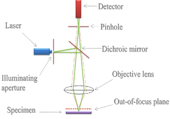
In CLSM, a beam of excitatory laser light from the illuminating aperture passes through an excitation filter and is reflected by a dichroic mirror to be focused by the microscope objective lens to a diffraction limited spot at the focal plane. 2-3,5,11 Fluorescence emissions excited both within the illuminated in-focus region, and within the illuminated cones above and below it, are collected by the objective and pass through the dichroic mirror and emission filter. However, only emissions from the in- focus region are able to pass through the confocal detector aperture, or pinhole, to be detected by the photomultiplier. This process is demonstrated schematically in Figure 1.2.10-11
In particular, fluorescence CLSM is a powerful and non-invasive in-situ technique which allows a 2D and 3D imaging of a sample.12-17 3D imaging of the sample may be constructed using a technique known as a z-stack illustrated in Figure 1.3. A 3D confocal image is created by collecting light from a single focal point of the sample at a time tracking many slices through the sample in the z-direction. These slices are then reconstituted into a three-dimensional picture by the software. A time series can be set
Specimen Slide
5 up so that an image or a z-stack can be taken at certain time intervals. This means that a reaction can be monitored over a particular time scale of interest.10
Figure 1.2: Schematic diagram of a confocal microscope.
6 Figure 1.3: Schematic of 3D z-stack imaging in CLSM.
Another important factor is the size of the pinhole. The smaller the pinhole used, the smaller the depth of focus. However, the use of very small pinholes may lead to darkening of the images because insufficient light can reach the detector. Thus, there is always a compromise between image clarity and pinhole size. Moreover, as discussed above, both fluorescent and reflected light from the sample pass back to a detector (photodiode system) through the objective in use. The objective lens parameters: (i) magnification, (ii) numerical aperture (NA) and (iii) free working distance, determine the resolution capacities of a given objective.3,5 The finest detail of the sample, that can be visualised with a microscope, is proportional to λ=NA (λ is the wavelength of the light).
1.1.3. Fluorescence
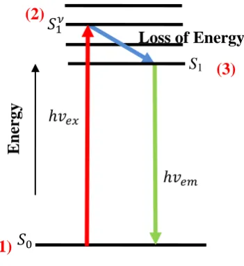
CLSM is particularly effective when fluorescent dyes are excited with the sharp band width of a laser. The fluorophores subsequently emit light of a sufficiently different wavelength to allow separation of the excitation and emission signals. The process involved in fluorescence is shown in a Jablonski diagram in Figure 1.4. A photon of
Stack
7 energy hνex excires an electron from the ground state of molecule (S0) (1) into vibrationally excited singlet state ( (2)(one or higher excited state of a higher energy).18-19 This excited state typically has a lifetime of 1-10 nanoseconds, and during this period the fluorophore may undergo conformational changes or be subject to possible interactions with its molecular environment. During these processes the energy of is partially dissipated to yield a relaxed singlet excited state, (3). Finally, a photon of energy hνem is emitted returning the fluorophore to its ground state, S0 (1).18
Figure 1.4: A Jablonski diagram showing the origin of fluorescence, with the photoexitation of an electron from (1) to (2) and emission light when the electron moves from (3) to (1).
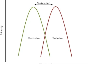
The difference between the positions of the band maxima of the excitation and emission wavelengths is known as the Stokes’ shift (see Figure 1.5). The wavelength of the
emitted light is characteristically longer than the wavelength of the absorbed light, as the energy of the emitted photon is lower due to the energy dissipation when the molecule is in the excited state. A large Stokes shift is a valuable attribute when trying
E
n
er
gy
S1 Loss of Energy (2)
(3)
[image:28.595.238.414.295.487.2]8 to detect the fluorescence since this means that the excitation and emitted photons can be easily distinguished and thus separated.
Figure 1.5: Definition of Stokes shift
1.1.3.1. Fluorescein
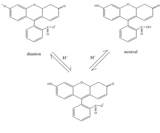
A molecule that is fluorescent is often called a fluorophore or a fluorescent dye. Fluorophores are fluorescent molecules which are usually polyaromatic hydrocarbons.20-21 They are generally used to label biological molecules and they respond to changes in their surroundings. A commonly used fluorophore, and one of particular relevance to this thesis, is fluorescein. Fluorescein is Bronsted-Lowry acid with a pKa 6.422 for the main ionization equilibrium of the mono and deprotonated form. The maximum excitation peak of fluorescein occurs at 494 nm; emission occurs only for the deprotonated form with maximum peak at 518 nm.3
Wavelength
Inte
nsit
y
9
(1.1)
Figure 1.6 (blue squares) shows a sigmoidal relationship of fluorescein fluorescence intensity (normalized) collected at the marked pH values.15,17 No fluorescence was observed below pH 5 and no increase in fluorescence occurred above pH 7. A calibration curve was obtained by a sigmoidal 3 parameter empirical fit.23
⁄
(1.2)
[image:30.595.160.504.286.528.2]where a and b are fitting parameters.
Figure 1.6: Illustration of intensity of fluorescence vs. pH after fluorescein excitation at
488 nm and detection at 530 nm.
10 fluorescence emission spectrum of fluorescein is dominated by the dianion with only small contribution from the monoanion until the pH falls below ca. 6.5 at which point the monanion becomes the prevalent species. The phenolic proton has a pKa of 6.5, whilst the carboxylic acid group has a pKa of 4.4.19 At very low pH, the quinine carbonyl group becomes protonated (pKa 2.1). Only the dianion is fluorescent, thus there is a sharp decrease in fluorescence at low pH where the neutral and cationic species dominate.
Figure 1.7: Molecular structures of neutral fluorescein and its anions.
The use of CLSM and fluorescein as a pH dependent probe of local pH is fundamental of much of the work in this thesis.
O O
HO
C
O OH
O O
HO
C
O O
O O
O
C
O O
dianion neutral
monoanion
11
1.2. Electrochemistry and Microelectrodes
1.2.1. Introduction to electrochemistry
The simplest electrode system is when a metal (or object) is placed in an electrolyte solution. This results in charge transfer at the interface between the electrode and the electrolyte, where gradients in electrical and chemical potentials constitute the driving force for electrochemical reactions. An electrical double layer forms 25-26 with the model outlined in Figure 1.8 showing a representation of the Grahame model. 27 This classical approach describes the electric double layer (EDL) of a metal electrolyte interface by a plate condenser of molecular dimensions. One plate is the metal surface with its excess charge; the other is formed by the solvated ions at closest approach. The solvated ions that form the outer Helmholtz plane (OHP) and that are held in position by purely electrostatic forces are termed “nonspecifically adsorbed”. These are mainly solvated
cations.
Most anions, however, if the electrode is positively charged give away part of that solvation shell when entering the double layer to form a chemical bond with the electrode surface. These ions are termed “specifically adsorbed” and their centres form
12 Figure 1.8: A diagrammatic representation of the electrical double layer where the red
cations are solvated with small blue circles representing water molecules, and large green anions are specifically adsorbed onto the electrode surface.
The double layer is frequently represented in an equivalent circuit as a capacitor. The current flowing due to the changing of the composition of the double layer is usually termed the charging current. It can limit the sensitivity of electrochemical measurements, particularly in a temporal sense. Also as the double layer can be thought of as a parallel plate capacitor, the size (spacing) is dependent on the concentration of electrolyte.25-26 High electrolyte concentrations reduce the size of this double layer.
1.2.2. Dynamic electrochemistry
13 reference electrode is chosen to have constant composition, and therefore a fixed potential.28 Where the typical current is expected to be greater than about 100 nA, a 3-electrode set-up is required. This introduction of a counter 3-electrode is necessary as such large currents would otherwise perturb the fixed potential of the reference electrode and render it unstable (due to electrolysis of its components).28
Measurement of the current that flows provides information on the solution, the electrodes and the interfacial reactions. The rate of the WE reaction is influenced by several factors, including the rate of the electron transfer at the electrode surface, mass transport of the redox-active species to the electrode, chemical reactions in the solution, the nature of the electrode surface, and the structure of the interfacial region over which the reaction occurs.
Figure 1.9: The effect of the applied potential on the Fermi level.27 Potential applied
Negative
Fermi level
Positive
Metal
Reactant
HOMO LUMO
14 The maximum of the continuum is known as the Fermi level. Application of a potential to the WE, with respect to the RE, can change the Fermi level of the metal used as the electrode (see Figure 1.9). While the Fermi level is of an energy between that of the lowest unoccupied molecular orbital (LUMO) and the highest occupied molecular orbital (HOMO), no electron transfer will occur. If a sufficiently negative potential is applied, the Fermi level increases in energy such that it is above the LUMO. In this situation, electron transfer occurs from the metal to the reactant, causing reduction of the reactant. Conversely, if a sufficiently positive potential is applied, the Fermi level decreases in energy such that it is below the HOMO. Electron transfer proceeds from the reactant to the metal electrode, leading to oxidation of the reactant.27
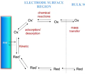
Figure 1.10: A schematic representation of a typical electrode reaction.28
15 or from the electrode. Under these conditions, the current response is limited by the rate of mass transport,27 which is the subject of the next section. More complex reactions may involve chemical reactions in solution, either before or after electron transfer, and surface reactions such as adsorption or desorption. Protonation is a common chemical reaction that is often coupled to electron transfer which leads to the production of pH gradients between the interfacial region and bulk solution, if the solution is not buffered. The aim of this thesis is to image and quantify the pH gradients that develop at active surfaces. These can arise either through chemical reactions in solution or electrode reactions that produce or consume protons or hydroxide ions, for example tris(2,2'-bipyridine)ruthenium(II) oxidation (chapter 3) and water oxidation (chapter 4 and 5).
1.2.3. Mass transport
Mass transfer of dilute species in solution is governed by the Nernst-Planck equation28 and for one-dimensional mass transfer along the x-axis the expression is as follows:
(1.3)
where Jjis the flux (i.e. the number of moles passing through a given area per unit time)
of species j to/from the electrode, Dj is the diffusion coefficient of species j, cj is the
concentration of species j, V is the velocity vector, zj is the charge on species j, F is the
Faraday’s constant, R is the gas constant, T is temperature and φ is the electrostatic
potential. The three terms on the right hand side represents the contributions of diffusion, convection, and migration, respectively, to the flux.25
16 carrying the species) and migration of the species (for example, the directed motion of ions due to some applied electrostatic potential).28 An increase in any of these factors can promote mass transport, alleviating them as a possible rate limiting factor in reactions with fast electrode surface kinetics. Addition of a background electrolyte to a cell minimises any effects from migration, and can aid eliminating the development of liquid junction potential and prevent any contributions from ohmic drop by decreasing the resistivity of the solution. The background electrolyte does not take part/ interfere in the reaction occurring at the tip of WE but does decreases the size of the double layer at the electrode/surface interface; where a small double layer results in a high electric field, ensuring that the full potential applied at the electrode is available for the electrochemical process.28-29
Experimental conditions can be chosen so that no significant contribution is made by convection and migration so that diffusion is dominant (as discussed above). Thus, all mass transport models of fluxes in this thesis make use of only the diffusive aspects of the Nernst- Planck equation, significantly simplifying any numerical analysis of experimental results. To precisely quantify electrode reactions, it is necessary to take each aspect of mass transport into consideration.
1.2.3.1. Diffusion
Diffusion is always present in a dynamic electrode process and is defined as the movement of a species down a concentration (formally, activity) gradient, due to the difference in concentration (activity) of the species at the electrode surface and the bulk solution. Diffusion is described mathematically by Fick’s laws28
17 (Equation 1.4) relates the diffusive flux to the concentration gradient (the rate of change of concentration with respect to distance).
(1.4)
where is the concentration gradient. The minus sign is because diffusion occurs down
a concentration gradient. Fick’s second law of diffusion describes the concentration of a
species varies with time.
(1.5)
where 2is the Laplace operator which is also geometry dependent. Of particular relevance to the studies described herein are the 1D equations.30
(1.6)
where c is the concentration, and x the distance over which the concentration changes. Solution of Fick’s second law can be used to give the variation in flux, or the
diffusion-limited current with time.
18 e.g. stirring), causing the reaction to become kinetically controlled as discussed in the next section.
1.2.3.2. Convection
Convection is the movement of species in a fluid due to an external mechanical force. The convective component of flux is given by:
(1.7)
There are two types of convection. The first is natural convection, which can be present in any solution and arises from thermal gradients and/or density differences within the solution. Forced convection is normally orders of magnitude larger than natural convection, and so obscures any effect that natural convection may have. It arises when the solution is deliberately agitated which can be achieved in several different ways, leading to a multitude of convective (or hydrodynamic) systems.31 In some electrochemical experiments an element of forced convection is deliberately introduced to swamp any contribution from natural convection, ensuring that reproducible experiments can be made over extended time-scales. Forced convection is usually achieved by external forces such as gas bubbling through solution, pumping, or stirring.28
1.2.3.3. Migration
From equation 1.1 it is apparent that migration only affects species which are charged. It is the movement of charged species under the influence of an external electric field (∂φ/∂x). Migrative flux is described by:
19 Due to the difficulty in quantifying its effect, migration is often removed during electrochemical experiments by the addition of an excess concentration of an inert supporting electrolyte.28 As already mentioned, this also has the benefit of reducing the effect of uncompensated (Ohmic) resistance and compressing the size of the electrical double layer, such that the potential across the electrode/solution interface drops over a distance commensurate with electron transfer.26,28 All studies in this thesis are carried out under conditions where migration can be ignored.
1.2.4 Ultramicroelectrodes (UMEs)
There are various types of electrodes employed and the critical factor determining their behaviour is the interplay between mass transport to the electrode and the electron transfer kinetics. The former may be directly linked to their size. Macroelectrodes have dimensions of the order of centimetres or millimetres; when one of the critical dimensions of the electrode is in the micrometer range, the electrode behaves as an ultramicroelectrode (UME).32-35
20 techniques and their application in the characterisation of UMEs are discussed in sections 1.2.5.1and 1.2.6, respectively.
The exposed part of the metal can take different forms (Figure 1.14),37,41 depending on the application42 and on the method of fabrication such as: disc electrodes,43 array, 44-45 band,46-47 hemisphere, cylinder, spherical mercury electrodes,48-49 ring electrodes,50-51 and carbon fibre electrodes52-53 ring,54-55 but by far the most widely used is the disc electrode since its fabrication is relatively straight forward, the sensing area can be polished mechanically and it is easily modellable. The diffusion fields, which promote the movement of materials to and from the electrode, are dependent on the shape of the electrode and the timescale of the measurement. Diffusion processes that take place are shown schematically in Figure 1.11. All show substantial “edge effects” which lead to
the enhanced mass transport rates.41
Figure 1.11: Different geometries of electrodes and their diffusion fields: (a) Disk
electrode (b) Cylinder electrode and (c) Ring electrode. Reproduced from reference.41
The size of the working electrode is an important consideration in electrochemical experiments. First, we should consider the traditional macroelectrode. Diffusion to this type of electrode is predominately planar, as shown in Figure 1.12(a). In contrast, the small size of UMEs results in extremely efficient diffusional mass transport due to the
Disc electrode Cylinder electrode Ring electrode
21 significant contribution of radial diffusion, resulting in the formation of a steady-state hemispherical diffusion field (in the case of a disc electrode). This is illustrated in Figure 1.12(b). Thus, more rapid and efficient mass transport occurs at a UME than that at a macroelectrode. This has important ramifications for the voltammetric response of UMEs, as discussed in section 1.2.5.
Thus, the use of UMEs allows fast kinetics to be observed and measured due to fast and well-defined mass transport properties as shown in Figure 1.12 28,55 In comparison to larger electrodes in quiescent solution, the advantage of a UME is its ability to form a steady-state current under diffusion controlled conditions.56 A small electrode area also results in a small charging current, allowing access to shorter time scales and fast response times. Small currents reduce effects from Ohmic drop, making UMEs effective in resistive media such as organic solutions, or in cases where electrolyte is not present.57
Figure 1.12: (a) Schematic of planar diffusion profile exhibited by a macroelectrode
and (b) the hemispherical diffusion at disc UME.
The UME tip is often characterised by the RG value, which is the ratio of the radius of insulating glass, rglass, to the electrode radius. It is defined as in equation (1.9), see
Figure 1.13. For most SECM studies RG is typically around 10. This minimizes effects
22 from back diffusion (from behind the probe), making the electrode response more sensitive to the surface process when used in SECM.
(1.9)
Figure 1.13: Showing the RG of an UME where rs is the radius of the whole UME and
a is the radius of the metal wire.
1.2.5. Linear Sweep Voltammetry and Cyclic Voltammetry
Linear Sweep Voltammetry (LSV) and Cyclic voltammetry (CV)58-59 are the simplest electrochemical techniques, and are used in most electrochemical investigations to provide information on the electrode/electrolyte interface. Consider the example electrode reaction O + e- → R. The basis of LSV is to ramp the potential linearly with time (V/s), at a particular scan rate. The potential increases from one where no reaction occurs, E1, to a potential were electron transfer is driven very quickly, E2. Upon
reaching E2, this will either oxidize or reduce an analyte of interest.
In CV, the direction of the sweep is reversed and the potential is scanned back to E1. If
the analyte of interest was reduced on the forward scan, the aim is that it may then be oxidised on the reverse scan, or vice-versa. This provides information on the reversibility of the reaction by analysis of the waveform produced; achieved by plotting the current recorded at the working electrode against the applied potential, as shown in Figure 1.14. At E1, no reduction occurs and so the current is zero. As the potential
a
23 increases, the rate of reduction increases, and so the current increases approximately exponentially with increasing potential (and thus time), as predicted by the Butler-Volmer equation.29 The current reaches a maximum value and a peak is seen. This occurs because the current depends not only on the rate constant for reduction, kred, but
also on the surface concentration of the redox species.
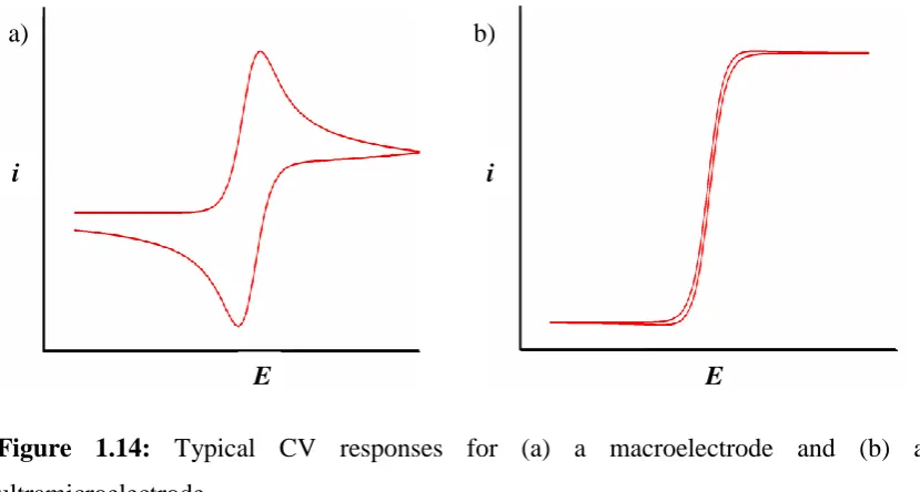
Figure 1.14: Typical CV responses for (a) a macroelectrode and (b) an
ultramicroelectrode.
Once this peak in the current is reached, the current is limited by the rate of mass transport (i.e. diffusion) of reactant to the electrode surface. The fall in current that occurs is due to an increase in the depth of the depleted region next to the electrode and the inability of mass transfer to compete with the rate of electron transfer. Once the sweep reaches the switching potential, E2, the potential reverses and the reaction
proceeds in the opposite direction. The voltammogram takes the form of a mirror image of the forward sweep, but is shifted by 59/n mV, as dictated by the Nernst equation for the case of a completely reversible.28 The scan rate plays an important role in the magnitude of the current. A typical voltammogram obtained for a macroelectrode is shown in Figure 1.14(a).
b) a)
i i
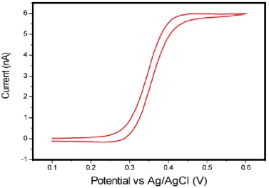
[image:44.595.115.530.222.444.2]24 The cyclic voltammogram observed for a UME takes a different form to that described above for a traditional macroelectrode (Figure 1.14) for relatively low scan rate. Instead of the peaked reponse, the voltammogram takes a sigmoidal shape, as shown in Figure 1.14(b). A maximum value of the current is observed, and the voltammogram plateaus at this value. This is termed the diffusion-limited current. This value of the current is maintained due to efficient replenishment of reactant at the electrode surface, resulting from rapid hemispherical diffusion to the UME. This bulk steady-state limiting current, for a disc UME can be theoretically calculated from Equation 1.10.25,60
(1.10)
where n is the number of electrons transferred in the electrode reaction, a is the electrode radius, c* is the bulk concentration of the electroactive species and K is a geometrydependent constant (K is 4 for a disc UME or 2π for a hemispherical UME).
Comparison of theoretical and experimental currents gives a quick indication that the system is working correctly. The shape of the sigmoidal waveform can be used to verify the electrode properties, e.g. the diameter of the active metal, the shape of the UME and how well the wire is sealed to the glass; and can be used to judge how good an electrode is. Both potential and scan rate can be controlled through a potentiostat, which monitors the potential applied to the tip and records the current response.
25
1.2.6. Scanning electrochemical microscopy (SECM)
SECM is a powerful scanned probe technique for quantitative investigations of interfacial physicochemical processes, in a wide variety of areas, as considered in several recent reviews.61-62 In the simplest terms, SECM involves the use of a mobile ultramicroelectrode (UME) probe, either amperometric or potentiometric, to investigate the activity and/or topography of an interface on a localized scale; typically resolution is on a micron length scale. It is capable of delivering a reagent to a surface with high rates of mass transport,28,63 and is highly controlled64-69 allowing the characterization of fast surface processes and the ability to study the chemical reactivity of analyte.70-79 A comprehensive review of all these aspects can be found in Bard and Mirkin.38
26 The advantages of SECM are that it is typically a non-invasive, non-destructive technique. It is well suited to small volumes where reactions can be detected directly and it allows the study of interfacial kinetic processes due to the high rates of mass transport achievable. It has high spatial resolution, versatility and selectivity. It is well known for chemical mapping and is used to investigate surface topography.81-82 As examples, the technique has been applied to air/water interfaces to study gas permeation,83 liquid/liquid interfaces,61,84-90 liquid/solid interfaces,68,91 single crystal, 65-67,92-93
and porous membranes.94-95
Chapter 4 and 5 outlines some further examples of SECM applications applicable to the work herein, in the fields of dissolution processes, kinetics and proton dispersion at many interfaces. Several modes of SECM have been developed to allow the local chemical properties of interfaces to be investigated. The mode of SECM most relevant to this work is the feedback mode.96 There are basically two forms: negative feedback and positive feedback.63 In this work, SECM is employed in the feedback mode to obtain approach curves to the surface of interest in order to determine UME-surface separation distance (chapters 4 and 5).
1.2.6.1 Negative Feedback
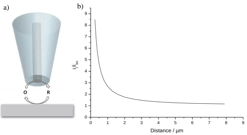
Negative feedback, where a UME approaches an insulating substrate, is shown in Figure 1.15(a). A potential is applied to the UME in order to reduce electroactive species O (present in solution) to species R at a diffusion limited rate, which generate a current, i∞,
27 begins to decrease in magnitude. This drop in current occurs at distances d < 10a. This is known as negative feedback.
Figure1.15: (a) Schematic of negative feedback, for an UME near an insulating
substrate and (b) Theoretical approach curve for a 25 µm diameter UME with an RG of 10, depicting negative feedback.
It is possible to plot curves showing it/i∞ vs d, where it is the current at the tip, it/i∞ is the
normalised current, and d is the distance between the electrode and the surface. These are known as approach curves. Theoretical approach curves may be constructed using the tables of Kwak and Bard96 and experimental data compared to them. A typical curve is shown in Figure 1.15 (b) for a 25 µm electrode with an RG of 10. This depicts a perfectly flat UME approaching an ideal insulator. As the electrode touches the surface, the flux of species is completely hindered and no current flows. However, in practice this is difficult to achieve and so a current of less than 10% of bulk at touch is considered sufficient (indicated by a point of inflection), i.e. the electrode and substrate are sufficiently well aligned and the UME is well polished.
0 10 20 30 40
0.0 0.2 0.4 0.6 0.8 1.0
it
/ilim
Distance / µm
28
1.2.6.2. Positive Feedback
Positive feedback63,96 occurs when the UME approaches a conducting substrate as shown in Figure 1.16 (a). In this situation, when the UME reaches a certain tip-surface separation, species R which has been generated at the tip is oxidised back to species O at the surface. This leads to an increasing concentration of species O being provided for reduction at the UME, and, as such, an increase in the current is seen. This is termed positive feedback. Theoretical approach curves for conducting surfaces can be plotted in a similar manner to those for insulating surfaces, discussed in section 2.2.1. The theoretical approach curve for a conducting substrate is given in Figure 1.16 (b) using a 25 µm diameter electrode with an RG of 10.
Figure 1.16: (a) Schematic of positive feedback near a conducting substrate (b)
Theoretical approach curve for a 25 µm diameter UME displaying positive feedback.
1.4. Finite Element Modelling (FEM)
The simulation in this thesis was performed using the commercially available software package, Comsol Multiphysics. This environment provides the user with all of the
0 1 2 3 4 5 6 7 8 9
0 1 2 3 4 5 6 7 8 9
it
/ilim
Distance / µm
[image:49.595.121.515.376.592.2]29 advantages of FEM, but a detailed knowledge of the complex mathematics behind this method is not required. It combines these advantages with an extremely user-friendly interface that enables simple construction of complex geometries (in one-, two- or three-dimensions) and simple definition of governing equations and boundary conditions. Many equations commonly used in the fields of engineering and physics are already built into the program (including diffusion, diffusion-convection and the Navier-Stokes equations for incompressible flow which are of relevance to this thesis) but a generic module is also present so that user defined equations can also be solved.
30 Figure 1.17: (a) An example of a simple triangular mesh used for FEM and (b) the
same domain where the mesh is finer at two edges.
Many systems have used finite element models as a means of aiding understanding of reactions processes, mechanisms or kinetics.97,102-103 In electrochemistry, FEM has been used both through self-written programs and commercially available software packages. In fact, one of the seminal SECM theory paper by Kwak and Bard,63 describing the positive and negative feedback response expected during an approach curve measurement, relied on finite element simulations. With particular relevance to SECM, models have been used to monitor transport through porous membranes, 104 to understand catalytic processes,105 and to develop tip positioning.106 Other researchers have used models to visualise the permeability of films107 and to define kinetics.108-109 For the work in this thesis and resulting publications, finite element models were created by a colleague, Dr. Martin Edwards to produce the theoretical characteristics and a fundamental understanding of the reaction processes occurring in solution. This aspect is described in more detail in Chapter 4 where boundary conditions and experimental parameters are also defined.
31
1.5. Aims of this Thesis
The overarching aim of thesis is to develop a new understanding of physiochemical processes and diffusion problems at interfaces by developing new techniques and exploring wider applications, which can be summarised as follows:
The main goal is to demonstrate the use of fluorescence CLSM coupled with electrochemical techniques and finite element modelling (through Comsol Multiphysics) in the quantification of concentration and pH gradients produced upon reaction at an electrode. The concentration gradient determined directly, while pH gradients are visualised through the addition of trace amounts of fluorescein, a dye that has a pH-dependent fluorescent signal. The fluorescence profile is predicted through simulation of the underlying mass transport equations.
Following on from the introduction, the apparatus used, experimental details and set-up are given in Chapter 2. This includes sample preparation, device microfabrication and characterisation, CLSM imaging experiments and the additional techniques used.
32 Chapter 4 describes the use of confocal microscopy coupled with SECM as a powerful technique for direct visualisation of acid-induced reaction processes and as a method for assessing the effectiveness of protective barriers on the enamel surface. It details the effect that fluoride and zinc treated enamel have on the prevention of acid attack. This found that Zn2+ treatment provides a much better barrier to prevent acid attack on enamel.
Chapter 5 investigates the lateral diffusion of protons through bilayer lipid membranes by the CLSM-SECM technique. A UME is brought close to the bilayer and galvanostatic water oxidation is induced, generating a proton gradient near the membrane. The transport of protons is observed as a pH change alongside bilayer. The effect of different ionisable head group, such as acidic distearoyl phosphatidylglycerol 1,2-ditetradecanoyl-sn-glycero-3-phospho-(1'-rac-glycerol) (DSPG) and zwitterionic phosphatidyl choline (EPC), on this process is also studied since it is thought that such negatively charged lipids facilitate proton lateral diffusion.