Preference Cloud Theory: Imprecise Preferences and Preference Reversals

(1)

Munich Personal RePEc Archive

Preference Cloud Theory: Imprecise

Preferences and Preference Reversals

Bayrak, Oben and Hey, John

Centre for Environmental and Resource Economics

2015

Online at

https://mpra.ub.uni-muenchen.de/71782/

(2)

Preference Cloud Theory: Imprecise Preferences and Preference Reversals Oben K. Bayrak and John D. Hey1

This paper presents a new theory, called Preference Cloud Theory, of

decision-making under uncertainty. This new theory provides an

explanation for empirically-observed Preference reversals. Central to the

theory is the incorporation of preference imprecision which arises because

of individuals’ vague understanding of numerical probabilities. We combine

this concept with the use of the Alpha model (which builds on Hurwicz’s

criterion) and construct a simple model which helps us to understand

various anomalies discovered in the experimental economics literature that

standard models cannot explain.

Key Words: Imprecise Preferences; Preference Reversals; Decision under Uncertainty; Anomalies in Expected Utility Theory

JEL Classification: D81

1

Oben K. Bayrak (corresponding author), PhD Candidate, Department of Forest Economics, SLU and CERE

(Center for Resource and Environmental Economics), Skogsmarksgränd, Umeå, 901 83, +46 727469175, [email protected]

John D. Hey, Professor, Department of Economics, University of York, Heslington, York, YO1 10DD,

(3)

1.

Introduction

Suppose you are asked to state your subjective value for a lottery ticket which gives 10 dollars with a

probability of 0.3 and zero otherwise: Can you pin your value down to a single precise number or do

you end up with a range of values? Our preference imprecision argument states that individuals

most likely end up having an interval; preferences are not as precise as standard theory presumes

(for evidence, see: Butler and Loomes, 1988, 2007, 2011; Dubourg et al, 1994, 1996; and Morrison,

1998). Such imprecision might explain observed anomalies of standard theory (Butler and Loomes

2011). Most importantly, imprecision might be the explanation of the anomalies, despite

researchers’ efforts, in the last four decades, focusing on precise but non-standard preferences such

as loss aversion.

Suppose now you are assigned to be a buyer. You are most likely to state a value close to the lower

bound of this range; the converse is true when you are assigned to be a seller. The model presented

in this paper answers two key questions: what is the psychological mechanism behind the formation

of this range?; how do individuals select one value from this range? It also shows how the

incorporation of imprecision can provide an explanation for preference reversals.

For the first question our theory proposes that imprecision arises due to the decision-maker’s vague

understanding of the probabilities involved. The empirical support for this assertion comes from the

psychophysics literature; see Budescu et al (1988). In an experiment reported by them subjects

were asked to state bids for lotteries; in the lotteries the probabilities were represented numerically,

graphically or verbally. The results suggested that bids and attractiveness ratings are almost identical

under the different representations (See Budescu and Wallsten (1990) and Bisantz et al (2005) for

further evidence). Wallsten and Budescu (1995) explain that the similarity of behavior under

different representation modes is due to similarities in the vague understanding of probabilities. We

(4)

subjects use this range in their calculations2. There is also implicit evidence from Plott and Zeiler

(2005) and Isoni et al (2011) who find that the endowment effect is observed only for the lottery

tickets, but not for ordinary market goods such as mugs and candies.

Zimmer (1984) introduced a useful insight from an evolutionary perspective: he noted that the

probability concept in a numerical sense is a relatively new concept, appearing as recently as the 17th

century. However, people were communicating uncertainty via verbal expressions long before

probability was codified in mathematical terms. Zimmer further suggested that people process

uncertainty in a verbal manner and make their decisions based on this processed information, not

on the numerical information. We therefore assume that decision makers map any given objective

probability into an interval. This implies that people end up with a range of expected utilities (EUs)

and they do not have prior knowledge about their “true” EU from this range. For the second

question, pinning down this range to a single value can be modelled as decision problem under

ambiguity. We use the Alpha Model (embodying Hurwicz’s criterion) to provide a valuation of the

prospect, given as the weighted average of the worst and the best possible EU. The next section

formalises these ideas.

2.

Theory

In order to give the intuition of the theory we focus on two-outcome lotteries. Let Sbe a finite state

space, with elements s₁ands₂; letx₁andx₂be the corresponding consequences. We assume that

   

1 2

u x u x , whereu

 

. is the individual’s Neumann-Morgenstern utility function. For each state

there is an objective probability; call thempand1p. The crucial point of our theory is that

individuals perceive these probabilities vaguely, and hencepis mapped to a range:



p,p



. As

far as the individual is concerned, the worst situation is when probabilityp is allocated to states₁

(5)

(and probability1 p  to states₂, and the best situation is when probabilityp is allocated to

states₁(and probability1 p to states₂). So the worst and best expected utilities are



p

   

u x1   1 p 

  

u x2 and



p

   

u x1   1 p 

  

u x2 respectively.

At this point PCT uses the Alpha Max-Min criterion to evaluate the lottery. This gives



   

1 1

   

2 1

 

   

1 1

  

2

EU p u x p u x p p u x p u x

   _     _    _     _ (1)

One can think of such a decision-maker as a mixture of a pessimist and an optimist:of the time he

or she assumes the worst, and1of the time the best.

The parameter we call the imprecision level; our theory postulates that it is a function ofp(the

objective probability) and (the individual-specific sophistication level). A relatively unsophisticated

individual would display a relatively high imprecision . For example, stock brokers and gamblers

who are expected to be more familiar with the concept of probability exhibit lower imprecision than

the ordinary man.

As far as the shape of 



,p



is concerned we assume that individuals exhibit no imprecision if the

probability is 0 or 1 since the events occurring with these probabilities are not probabilistic events in

daily language, that is, the event either never happens or always happens. Secondly, imprecision

reaches a maximum at 0.5 because it implies the event is neither likely nor unlikely, this

‘incommensurability’ makes it difficult to derive a meaning from this probability. Finally, for

simplicity we assume that 



,p



is symmetric aroundp0.5.

3.

Explaining Preference Reversals

We show how preference reversals can arise with our model. We illustrate using the CRRA utility

function foru

 

.

( ) a

(6)

Fora0, the function is concave, implying risk aversion. For simplicity, we focus on P and $ bets

that give either a positive payoff or zero: P-bet



x p, ;0



and $-bet



y q, ;0



withy x 0and

1  p q 0 wherep and q are the winning probabilities, andxandyare the winning prizes of the

P-bet and $-bet, respectively.

If the individual prefers the P-bet over the $-bet in the choice task, we can write:







$



EU P bet EU bet

    (2)





a



1

 



a





a



1





a

p x p x q y p y

_  _  _  __  _   (3)

Thus the critical value for in determining whether the P-bet preferred to the $-bet is:













* 2 a a a a

y q x p

y x        

 (4)

If the actualis greater than*the individual chooses the P-bet; if lower the $-bet.

When we come to valuations we need to tell a different story. Let us consider willingness-to-accept.

Take the P-bet. Imagine that the individual owns the P-bet and is asked the minimum amount for

which he or she would sell it – the WTA. If it is sold the individual has WTA (presumably an amount

less thanx), and the worst thing that can ‘happen’ to the individual is that the P-bet would have

paid outx, and the best thing that can ‘happen’ to the individual is that the P-bet would have paid

out 0. So the pessimist attaches weightpto the possibility of gettingx, while the optimist

attaches weightp . So we get











 



1 a ₁ a

P bet

u WTA _ _ p x _  _ p x _ (5)

Similarly,











 



1 $ 1 a a bet

u WTA _ _ q y _  _ q y _ (6)

(7)













** 2 a a a a

x p y q

y x        

 (7)

Ifis greater**the individual values the $-bet higher than the P-bet; if it is lower the P-bet is

valued higher.

We explore the parameters of PCT in three cases: risk neutral, risk averse and a risk loving. Consider

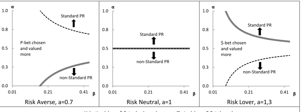
[image:7.595.48.552.290.478.2]

Figure 2, where r set to 1; P-bet



1.25,0.8;0 ,



$-bet



5,0.2;0



3

Figure 1

Risk Averse, a=0.7 Risk Neutral, a=1 Risk Lover, a=1,3

The dashed line shows the**boundary and the solid line is the*boundary. Above the dashed

line the $-bet is valued higher and above the solid gray line the P-bet is chosen; the region between

the two lines is called the consistency range where the chosen bet is valued more. For a risk-neutral

individual, in the case of imprecision(0),a standard Preference reversal occurs if 0.5, when it

is lower than 0.5, the model predicts a non-standard Preference reversal. For a risk-averse

individual, in the consistency range individual chooses the P-Bet and values it higher; whereas for

the risk loving case the $-Bet is chosen and valued more. This makes sense: the P-bet would be more

3

For the imprecision level, we use  

 

,p p



1p



, there is no particular reason behind choosing this, except it is simple and satisfies the assumptions of the theory. We normalize the expected value (EV) of the P bet by setting its payoff equal to1 / ;p ris the EV of the $ bet as a ratio of the EV of the P-bet. Therefore the winning prize of the $ bet equalsr/ .p

0.0 0.3 0.5 0.8 1.0

0.01 0.21 0.41

α β Standard PR

non-Standard PR P-bet chosen and valued more 0.0 0.3 0.5 0.8 1.0

0.01 0.21 0.41

α β Standard PR

non-Standard PR 0.0 0.3 0.5 0.8 1.0

0.01 0.21 0.41

α β Standard PR

non-Standard PR $-bet chosen and valued more 0.0 0.3 0.5 0.8 1.0

(8)

attractive for a risk-averse individual. Overall, in the case of imprecision( 0),a sufficiently high

level of pessimism results in a standard Preference Reversal while optimism implies a non-standard

Preference Reversal.

Next we consider the case in which the winning probabilities remain the same, but the winning prize

[image:8.595.158.440.276.462.2]

of the $-Bet varies. Figure 3 shows the critical bounds for three cases:

Figure 2

Risk Averse, a=0.7

The dashed lines show the valuation boundary, and the solid lines show the choice boundary, for

three levels of r(0.8,1,1.2). For a risk-averse decision-maker, the consistency range shrinks asr

increases up to a certain level. The parameter values to induce standard and non-standard

preference reversals converge to the risk neutrality baseline case. However, above this critical level

ofr,the consistency range favors the $-bet and it expands asrincreases. Even if we increase the

relative attractiveness of the $-bet to extreme values, the model predicts that both standard and

non-standard preference reversals can be observed. 0.0

0.3 0.5 0.8 1.0

0.01 0.21 0.41

α

β

Standard PR

non-Standard PR Consistency

Range

0 1

0 0.5 1

Valuation (r=0.8)

Valuation (r=1)

Valuation (r=1.2)

Choice (r=0.8)

Choice (r=1)

(9)

4.

Conclusion

We demonstrated the intuition of the Preference Cloud Theory and explained the possible

preference reversals. In the same manner other anomalies of EUT can be explained such as

Endowment Effect and Allais Paradox. To best of our knowledge, this is the only theory that can

explain anomalies in Expected Utility theory without incorporating the loss aversion notion of the

(10)

REFERENCES

Arrow, Kenneth J. and Leonid Hurwicz, “An Optimality Criterion for Decision-Making under Ignorance.” In

Carter, C. F. and J. L. Ford, eds., Uncertainty and Expectations in Economics. Oxford: Basil Blackwell,

1972.

Bisantz, Ann M., Stephanie Schinzing Marsiglio, and Jessica Munch. 2005. “Displaying Uncertainty:

Investigating the Effects of Display Format and Specificity.” Human Factors: The Journal of the

Human Factors and Ergonomics Society 47 (4): 777–96.

Budescu, David V., Shalva Weinberg, and Thomas S. Wallsten. 1988. “Decisions Based on Numerically and

Verbally Expressed Uncertainties.” Journal of Experimental Psychology: Human Perception and

Performance 14 (2): 281.

Budescu, David V., and Thomas S. Wallsten. 1990. “Dyadic Decisions with Numerical and Verbal

Probabilities.” Organizational Behavior and Human Decision Processes 46 (2): 240–63.

Butler, David, and Graham Loomes. 1988. “Decision Difficulty and Imprecise Preferences.” Acta

Psychologica 68 (1–3): 183–96.

Butler, David J., and Graham C. Loomes. 2007. “Imprecision as an Account of the Preference Reversal

Phenomenon.” American Economic Review 97 (1): 277–97.

Butler, David, and Graham Loomes. 2011. “Imprecision as an Account of Violations of Independence and

Betweenness.” Journal of Economic Behavior & Organization 80 (3): 511–22.

Dubourg, W. R., M. W. Jones-Lee, and Graham Loomes. 1994. “Imprecise Preferences and the WTP-WTA

Disparity.” Journal of Risk and Uncertainty 9 (2): 115–33.

Dubourg, Jones-Lee, and Graham Loomes. 1997. “Imprecise Preferences and Survey Design in Contingent

(11)

Isoni, Andrea, Graham Loomes, and Robert Sugden. “The Willingness to Pay Willingness to Accept Gap,

the Endowment Effect, Subject Misconceptions, and Experimental Procedures for Eliciting

Valuations: Comment.” The American Economic Review 101, no. 2 (2011): 991–1011.

Morrison, Gwendolyn C. 1998. “Understanding the Disparity between WTP and WTA: Endowment Effect,

Substitutability, or Imprecise Preferences?” Economics Letters 59 (2): 189–94.

Plott, Charles R., and Kathryn Zeiler. “The Willingness to Pay-Willingness to Accept Gap, the ‘Endowment

Effect,’ Subject Misconceptions, and Experimental Procedures for Eliciting Valuations.” The American

Economic Review 95, no. 3 (June 1, 2005): 530–45.

Wallsten, Thomas S, Samuel Fillenbaum, and James A Cox. 1986. “Base Rate Effects on the Interpretations

of Probability and Frequency Expressions.” Journal of Memory and Language 25 (5): 571–87.

Wallsten, Thomas S., and David V. Budescu. 1995. “A Review of Human Linguistic Probability Processing:

General Principles and Empirical Evidence.” The Knowledge Engineering Review 10 (01): 43–62.

Zimmer, Alf C. 1984. “A Model for the Interpretation of Verbal Predictions.” International Journal of