Incremental HMM Alignment for MT System Combination
Chi-Ho Li
Microsoft Research Asia 49 Zhichun Road, Beijing, China
Xiaodong He
Microsoft Research
One Microsoft Way, Redmond, USA
Yupeng Liu
Harbin Institute of Technology 92 Xidazhi Street, Harbin, China
Ning Xi
Nanjing University 8 Hankou Road, Nanjing, China
Abstract
Inspired by the incremental TER align-ment, we re-designed the Indirect HMM (IHMM) alignment, which is one of the best hypothesis alignment methods for conventional MT system combination, in an incremental manner. One crucial prob-lem of incremental alignment is to align a hypothesis to a confusion network (CN). Our incremental IHMM alignment is im-plemented in three different ways: 1) treat CN spans as HMM states and define state transition as distortion over covered n -grams between two spans; 2) treat CN spans as HMM states and define state tran-sition as distortion over words in compo-nent translations in the CN; and 3) use a consensus decoding algorithm over one hypothesis and multiple IHMMs, each of which corresponds to a component trans-lation in the CN. All these three ap-proaches of incremental alignment based on IHMM are shown to be superior to both incremental TER alignment and conven-tional IHMM alignment in the setting of the Chinese-to-English track of the 2008 NIST Open MT evaluation.
1 Introduction
Word-level combination using confusion network (Matusov et al. (2006) and Rosti et al. (2007)) is a widely adopted approach for combining Machine Translation (MT) systems’ output. Word align-ment between a backbone (or skeleton) translation and a hypothesis translation is a key problem in this approach. Translation Edit Rate (TER, Snover et al. (2006)) based alignment proposed in Sim
et al. (2007) is often taken as the baseline, and a couple of other approaches, such as the Indi-rect Hidden Markov Model (IHMM, He et al. (2008)) and the ITG-based alignment (Karakos et al. (2008)), were recently proposed with better re-sults reported. With an alignment method, each hypothesis is aligned against the backbone and all the alignments are then used to build a confusion network (CN) for generating a better translation.
However, as pointed out by Rosti et al. (2008), such a pair-wisealignment strategy will produce a low-quality CN if there are errors in the align-ment of any of the hypotheses, no matter how good the alignments of other hypotheses are. For ex-ample, suppose we have the backbone “he buys a computer” and two hypotheses “he bought a lap-top computer” and “he buys a laplap-top”. It will be natural for most alignment methods to produce the alignments in Figure 1a. The alignment of hypoth-esis 2 against the backbone cannot be considered an error if we consider only these two translations; nevertheless, when added with the alignment of another hypothesis, it produces the low-quality CN in Figure 1b, which may generate poor trans-lations like “he bought a laptop laptop”. While it could be argued that such poor translations are un-likely to be selected due to language model, this CN does disperse the votes to the word “laptop” to two distinct arcs.
Rosti et al. (2008) showed that this problem can be rectified by incremental alignment. If hypoth-esis 1 is first aligned against the backbone, the CN thus produced (depicted in Figure 2a) is then aligned to hypothesis 2, giving rise to the good CN as depicted in Figure 2b.1 On the other hand, the
1Note that this CN may generate an incomplete sentence
“he bought a”, which is nevertheless unlikely to be selected as it leads to low language model score.
Figure 1: An example bad confusion network due to pair-wise alignment strategy
correct result depends on the order of hypotheses. If hypothesis 2 is aligned before hypothesis 1, the final CN will not be good. Therefore, the obser-vation in Rosti et al. (2008) that different order of hypotheses does not affect translation quality is counter-intuitive.
This paper attempts to answer two questions: 1) as incremental TER alignment gives better perfor-mance than pair-wise TER alignment, would the incremental strategy still be better than the pair-wise strategy if the TER method is replaced by another alignment method? 2) how does transla-tion quality vary for different orders of hypotheses being incrementally added into a CN? For ques-tion 1, we will focus on the IHMM alignment method and propose three different ways of imple-menting incremental IHMM alignment. Our ex-periments will also try several orders of hypothe-ses in response to question 2.
This paper is structured as follows. After set-ting the notations on CN in section 2, we will first introduce, in section 3, two variations of the basic incremental IHMM model (IncIHMM1 and IncIHMM2). In section 4, a consensus decoding algorithm (CD-IHMM) is proposed as an alterna-tive way to search for the optimal alignment. The issues of alignment normalization and the order of hypotheses being added into a CN are discussed in sections 5 and 6 respectively. Experiment results and analysis are presented in section 7.
Figure 2: An example good confusion network due to incremental alignment strategy
2 Preliminaries: Notation on Confusion Network
Before the elaboration of the models, let us first clarify the notation on CN. A CN is usually de-scribed as a finite state graph with many spans. Each span corresponds to a word position and con-tains several arcs, each of which represents an al-ternative word (could be the empty symbol ,²) at that position. Each arc is also associated withM weights in an M-way system combination task. Follow Rosti et al. (2007), the i-th weight of an arc isPr1+1r, whereris the rank of the hypothe-sis in thei-th system that votes for the word repre-sented by the arc. This conception of CN is called theconventionalorcompactform of CN. The net-works in Figures 1b and 2b are examples.
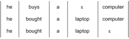
On the other hand, as a CN is an integration of the skeleton and all hypotheses, it can be con-ceived as a list of the component translations. For example, the CN in Figure 2b can be converted to the form in Figure 3. In such an expanded or
[image:2.595.70.288.69.282.2]Figure 3: An example of confusion network in tab-ular form
rank-based weights from different system can be compared to each other without adjustment. The weight of a cell is the same as the weight of the corresponding row. In this paper the elaboration of the incremental IHMM models is based on such tabular form of CN.
LetEI
1 = (E1. . . EI)denote the backbone CN,
and e01J = (e01. . . e0J) denote a hypothesis being aligned to the backbone. Eache0
j is simply a word
in the target language. However, eachEiis a span, or a column, of the CN. We will also useE(k)to denote the k-th row of the tabular form CN, and Ei(k) to denote the cell at the k-th row and the
i-th column. W(k) is the weight for E(k), and Wi(k) = W(k) is the weight for Ei(k). pi(k)
is the normalized weight for the cellEi(k), such
thatpi(k) = PWi(k)
iWi(k)
. Note that E(k) contains the same bag-of-words as the k-th original trans-lation, but may have different word order. Note also that E(k) represents a word sequence with inserted empty symbols; the sequence with all in-serted symbols removed is known as thecompact
form ofE(k).
3 The Basic IncIHMM Model
A na¨ıve application of the incremental strategy to IHMM is to treat a span in the CN as an HMM state. Like He et al. (2008), the conditional prob-ability of the hypothesis given the backbone CN can be decomposed into similarity model and dis-tortion model in accordance with equation 1
p(e01J|E1I) =X
aJ
1
J
Y
j=1
[p(aj|aj−1, I)p(e0j|eaj)] (1)
The similarity between a hypothesis word e0j and a spanEiis simply a weighted sum of the
similar-ities betweene0
j and each word contained inEias
equation 2:
p(e0j|Ei) =
X
Ei(k)²Ei
pi(k)·p(e0j|Ei(k)) (2)
The similarity between two words is estimated in exactly the same way as in conventional IHMM alignment.
As to the distortion model, the incremental IHMM model also groups distortion parameters into a few ‘buckets’:
c(d) = (1 +|d−1|)−K
The problem in incremental IHMM is when to ap-ply a bucket. In conventional IHMM, the transi-tion from stateitojhas probability:
p0(j|i, I) = PIc(j−i)
l=1c(l−i)
(3)
It is tempting to apply the same formula to the transitions in incremental IHMM. However, the backbone in the incremental IHMM has a special property that it is gradually expanding due to the insertion operator. For example, initially the back-bone CN contains the optioneiin thei-th span and
the optionei+1in the(i+1)-th span. After the first round alignment, perhapsei is aligned to the
hy-pothesis worde0
j,ei+1toe0j+2, and the hypothesis
worde0
j+1is left unaligned. Then the consequent
CN have an extra span containing the optione0j+1 inserted between thei-th and(i+ 1)-th spans of the initial CN. If the distortion buckets are applied as in equation 3, then in the first round alignment, the transition from the span containingei to that
containing ei+1 is based on the bucket c(1), but
in the second round alignment, the same transition will be based on the bucketc(2). It is therefore not reasonable to apply equation 3 to such gradually extending backbone as the monotonic alignment assumption behind the equation no longer holds.
There are two possible ways to tackle this prob-lem. The first solution estimates the transition probability as a weighted average of different dis-tortion probabilities, whereas the second solution converts the distortion over spans to the distortion over the words in each hypothesisE(k)in the CN.
3.1 Distortion Model 1: simple weighting of covered n-grams
Distortion Model 1 shifts the monotonic alignment assumption from spans of CN to n-grams covered by state transitions. Let us illustrate this point with the following examples.
In conventional IHMM, the distortion probabil-ity p0(i+ 1|i, I) is applied to the transition from
jumps across only one word, viz. thei-th word of the backbone. In incremental IHMM, suppose the i-th span covers two arcseaand², with
probabili-tiesp1andp2= 1−p1respectively, then the
tran-sition from stateitoi+ 1jumps across one word (ea) with probabilityp1 and jumps across nothing
with probabilityp2. Thus the transition
probabil-ity should bep1·p0(i+ 1|i, I) +p2·p0(i|i, I).
Suppose further that the(i+ 1)-th span covers two arcseband², with probabilitiesp3andp4
re-spectively, then the transition from stateitoi+ 2 covers 4 possible cases:
1. nothing (²²) with probabilityp2·p4;
2. the unigrameawith probabilityp1·p4;
3. the unigrameb with probabilityp2·p3;
4. the bigrameaebwith probabilityp1·p3.
Accordingly the transition probability should be
p2p4p0(i|i, I) +p1p3p0(i+ 2|i, I) +
(p1p4+p2p3)p0(i+ 1|i, I).
The estimation of transition probability can be generalized to any transition from i to i0 by ex-panding all possiblen-grams covered by the tran-sition and calculating the corresponding probabil-ities. We enumerate all possible cell sequences S(i, i0) covered by the transition from span i to
i0; each sequence is assigned the probability
Pii0 =
i0−1
Y
q=i
pq(k).
where the cell at the i0-th span is on some row
E(k). Since a cell may represent an empty word, a cell sequence may represent an n-gram where 0 ≤ n ≤ i0−i(or0 ≤ n ≤ i−i0 in backward
transition). We denote|S(i, i0)|to be the length of
n-gram represented by a particular cell sequence S(i, i0). All the cell sequencesS(i, i0)can be
clas-sified, with respect to the length of corresponding n-grams, into a set of parameters where each ele-ment (with a particular value ofn) has the proba-bility
Pii0(n;I) = X
|S(i,i0)|=n
Pii0.
The probability of the transition fromitoi0 is:
p(i0|i, I) =X
n
[Pii0(n;I)·p0(i+n|i, I)]. (4)
That is, the transition probability of incremental IHMM is a weighted sum of probabilities of ‘n-gram jumping’, defined as conventional IHMM distortion probabilities.
However, in practice it is not feasible to ex-pand all possiblen-grams covered by any transi-tion since the number ofn-grams grows exponen-tially. Therefore a length limitLis imposed such that for all state transitions where|i0−i| ≤L, the
transition probability is calculated as equation 4, otherwise it is calculated by:
p(i0|i, I) = max
q p(i
0|q, I)·p(q|i, I)
for someq betweeniandi0. In other words, the
probability of longer state transition is estimated in terms of the probabilities of transitions shorter or equal to the length limit.2 All the state transi-tions can be calculated efficiently by dynamic pro-gramming.
A fixed value P0 is assigned to transitions to null state, which can be optimized on held-out data. The overall distortion model is:
˜
p(j|i, I) = (
P0 ifjis null state
(1−P0)p(j|i, I) otherwise
3.2 Distortion Model 2: weighting of distortions of component translations
The cause of the problem of distortion over CN spans is the gradual extension of CN due to the inserted empty words. Therefore, the problem will disappear if the inserted empty words are re-moved. The rationale of Distortion Model 2 is that the distortion model is defined over the ac-tual word sequence in each component translation E(k).
Distortion Model 2 implements a CN in such a way that therealposition of thei-th word of thek -th component translation can always be retrieved. The real position of Ei(k), δ(i, k), refers to the
position of the word represented by Ei(k) in the
compact form ofE(k)(i.e. the form without any inserted empty words), or, ifEi(k)represents an
empty word, the position of the nearest preceding non-empty word. For convenience, we also denote by δ²(i, k) the null state associated with the state
of the real wordδ(i, k). Similarly, the real length
2This limitLis also imposed on the parameterIin
distor-tion probabilityp0(i0|i, I), because the value ofIis growing
ofE(k),L(k), refers to the number of non-empty words ofE(k).
The transition from spani0 toiis then defined as
p(i|i0) = P 1
kW(k)
X
k
[W(k)·pk(i|i0)] (5)
wherekis the row index of the tabular form CN. Depending on Ei(k) and Ei0(k), pk(i|i0) is
computed as follows:
1. if both Ei(k) and Ei0(k) represent real
words, then
pk(i|i0) =p0(δ(i, k)|δ(i0, k), L(k))
where p0 refers to the conventional IHMM distortion probability as defined by equa-tion 3.
2. ifEi(k)represents a real word butEi0(k)the
empty word, then
pk(i|i0) =p0(δ(i, k)|δ²(i0, k), L(k))
Like conventional HMM-based word align-ment, the probability of the transition from a null state to a real word state is the same as that of the transition from the real word state associated with that null state to the other real word state. Therefore,
p0(δ(i, k)|δ
²(i0, k), L(k)) =
p0(δ(i, k)|δ(i0, k), L(k))
3. if Ei(k) represents the empty word but
Ei0(k)a real word, then
pk(i|i0) =
(
P0 ifδ(i, k) =δ(i0, k)
P0Pδ(i|i0;k) otherwise
wherePδ(i|i0;k) =p0(δ(i, k)|δ(i0, k), L(k)).
The second option is due to the constraint that a null state is accessible only to itself or the real word state associated with it. Therefore, the transition fromi0toiis in fact composed
of the first transition fromi0toδ(i, k)and the
second transition fromδ(i, k)to the null state ati.
4. if bothEi(k)andEi0(k)represent the empty
word, then, with similar logic as cases 2 and 3,
pk(i|i0) = (
P0 ifδ(i, k) =δ(i0, k)
P0Pδ(i|i0;k) otherwise
4 Incremental Alignment using Consensus Decoding over Multiple IHMMs
The previous section describes an incremental IHMM model in which the state space is based on the CN taken as a whole. An alternative approach is to conceive the rows (component translations) in the CN as individuals, and transforms the align-ment of a hypothesis against an entire network to that against the individual translations. Each in-dividual translation constitutes an IHMM and the optimal alignment is obtained from consensus de-coding over these multiple IHMMs.
Alignment over multiple sequential patterns has been investigated in different contexts. For ex-ample, Nair and Sreenivas (2007) proposed multi-pattern dynamic time warping (MPDTW) to align multiple speech utterances to each other. How-ever, these methods usually assume that the align-ment is monotonic. In this section, a consensus decoding algorithm that searches for the optimal (non-monotonic) alignment between a hypothesis and a set of translations in a CN (which are already aligned to each other) is developed as follows.
A prerequisite of the algorithm is a function for converting a span index to the corresponding HMM state index of a component translation. The two functionsδandδ²s defined in section 3.2 are
used to define a new function:
¯
δ(i, k) = (
δ²(i, k) ifEi(k)is null
δ(i, k) otherwise
Accordingly, given the alignmentaJ
1 = a1. . . aJ
of a hypothesis (with J words) against a CN (where each aj is an index referring to the span
of the CN), we can obtain the alignment ˜ak = ¯
δ(a1, k). . .δ(a¯ J, k) between the hypothesis and the k-th row of the tabular CN. The real length functionL(k)is also used to obtain the number of non-empty words ofE(k).
Given the k-th row of a CN, E(k), an IHMM λ(k)is formed and the cost of the pair-wise align-ment,˜ak, between a hypothesishandλ(k)is de-fined as:
C( ˜ak;h, λ(k)) =−logP(˜ak|h, λ(k)) (6)
The cost of the alignment ofhagainst a CN is then defined as the weighted sum of the costs of the K alignments˜ak:
C(a;h,Λ) = X
k
= −X k
W(k) logP(˜ak|h, λ(k))
whereΛ ={λ(k)}is the set of pair-wise IHMMs, andW(k)is the weight of thek-th row. The op-timal alignment aˆ is the one that minimizes this cost:
ˆ
a = arg max
a
X
k
W(k) logP(˜ak|h, λ(k))
= arg max
a
X
k
W(k)[X
j
[
logP(¯δ(aj, k)|δ(a¯ j−1, k), L(k)) +
logP(ej|Ei(k))]] = arg max
a
X
j
[
X
k
W(k) logP(¯δ(aj, k)|¯δ(aj−1, k), L(k)) +
X
k
W(k) logP(ej|Ei(k))]
= arg max
a
X
j
[logP0(aj|aj−1) +
logP0(ej|Eaj)]
A Viterbi-like dynamic programming algorithm can be developed to search for ˆaby treating CN spans as HMM states, with a pseudo emission probability as
P0(ej|Eaj) =
K
Y
k=1
P(ej|Eaj(k))W(k)
and a pseudo transition probability as
P0(j|i) =
K
Y
k=1
P(¯δ(j, k)|δ(i, k), L(k))¯ W(k)
Note that P0(ej|Eaj) and P0(j|i) are not true probabilities and do not have the sum-to-one prop-erty.
5 Alignment Normalization
After alignment, the backbone CN and the hypoth-esis can be combined to form an even larger CN. The same principles and heuristics for the con-struction of CN in conventional system combina-tion approaches can be applied. Our incremen-tal alignment approaches adopt the same heuris-tics for alignment normalization stated in He et al. (2008). There is one exception, though. All 1-N mappings are not converted toN −1²-1 map-pings since this conversion leads toN −1
inser-tion in the CN and therefore extending the net-work to an unreasonable length. The Viterbi align-ment is abandoned if it contains an 1-N mapping. The best alignment which contains no 1-N map-ping is searched in the N-Best alignments in a way inspired by Nilsson and Goldberger (2001). For example, if both hypothesis wordse0
1 ande02 are
aligned to the same backbone span E1, then all
alignments aj={1,2} = i (where i 6= 1) will be examined. The alignment leading to the least re-duction of Viterbi probability when replacing the alignmentaj={1,2}= 1will be selected.
6 Order of Hypotheses
The default order of hypotheses in Rosti et al. (2008) is to rank the hypotheses in descending of their TER scores against the backbone. This pa-per attempts several other orders. The first one is
system-basedorder, i.e. assume an arbitrary order of the MT systems and feeds all the translations (in their original order) from a system before the translations from the next system. The rationale behind the system-based order is that the transla-tions from the same system are much more similar to each other than to the translations from other systems, and it might be better to build CN by incorporating similar translations first. The sec-ond one isN-best rank-basedorder, which means, rather than keeping the translations from the same system as a block, we feed the top-1 translations from all systems in some order of systems, and then the second best translations from all systems, and so on. The presumption of the rank-based or-der is that top-ranked hypotheses are more reliable and it seemed beneficial to incorporate more reli-able hypotheses as early as possible. These two kinds of order of hypotheses involve a certain de-gree of randomness as the order of systems is arbi-trary. Such randomness can be removed by impos-ing aBayes Riskorder on MT systems, i.e. arrange the MT systems in ascending order of the Bayes Risk of their top-1 translations. These four orders of hypotheses are summarized in Table 1. We also tried some intuitively bad orders of hypotheses, in-cluding the reversalof these four orders and the random order.
7 Evaluation
Order Example
System-based 1:1 . . . 1:N 2:1 . . . 2:N . . . M:1 . . . M:N
[image:7.595.72.467.61.133.2]N-best Rank-based 1:1 2:1 . . . M:1 . . . 1:2 2:2 . . . M:2 . . . 1:N . . . M:N Bayes Risk + System-based 4:1 4:2 . . . 4:N . . . 1:1 1:2 . . . 1:N . . . 5:1 5:2 . . . 5:N Bayes Risk + Rank-based 4:1 . . . 1:1 . . . 5:1 4:2 . . . 1:2 . . . 5:2 . . . 4:N . . . 1:N . . . 5:N
Table 1: The list of order of hypothesis and examples. Note that ‘m:n’ refers to then-th translation from them-th system.
Evaluation (NIST (2008)). In the following sec-tions, the incremental IHMM approaches using distortion model 1 and 2 are named as IncIHMM1 and IncIHMM2 respectively, and the consensus decoding of multiple IHMMs as CD-IHMM. The baselines include the TER-based method in Rosti et al. (2007), the incremental TER method in Rosti et al. (2008), and the IHMM approach in He et al. (2008). The development (dev) set comprises the newswire and newsgroup sections of MT06, whereas the test set is the entire MT08. The 10-best translations for every source sentence in the dev and test sets are collected from eight MT sys-tems. Case-insensitive BLEU-4, presented in per-centage, is used as evaluation metric.
The various parameters in the IHMM model are set as the optimal values found in He et al. (2008). The lexical translation probabilities used in the semantic similarity model are estimated from a small portion (FBIS + GALE) of the constrained track training data, using standard HMM align-ment model (Och and Ney (2003)). The back-bone of CN is selected by MBR. The loss function used for TER-based approaches is TER and that for IHMM-based approaches is BLEU. As to the incremental systems, the default order of hypothe-ses is the ascending order of TER score against the backbone, which is the order proposed in Rosti et al. (2008). The default order of hypotheses for our three incremental IHMM approaches is N-best rank order with Bayes Risk system order, which is empirically found to be giving the high-est BLEU score. Once the CN is built, the final system combination output can be obtained by de-coding it with a set of features and dede-coding pa-rameters. The features we used include word con-fidences, language model score, word penalty and empty word penalty. The decoding parameters are trained by maximum BLEU training on the dev set. The training and decoding processes are the same as described by Rosti et al. (2007).
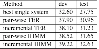
Method dev test
[image:7.595.308.481.187.272.2]best single system 32.60 27.75 pair-wise TER 37.90 30.96 incremental TER 38.10 31.23 pair-wise IHMM 38.52 31.65 incremental IHMM 39.22 32.63
Table 2: Comparison between IncIHMM2 and the three baselines
7.1 Comparison against Baselines
Table 2 lists the BLEU scores achieved by the three baseline combination methods and IncIHMM2. The comparison between pairwise and incremental TER methods justifies the supe-riority of the incremental strategy. However, the benefit of incremental TER over pair-wise TER is smaller than that mentioned in Rosti et al. (2008), which may be because of the difference between test sets and other experimental conditions. The comparison between the two pair-wise alignment methods shows that IHMM gives a 0.7 BLEU point gain over TER, which is a bit smaller than the difference reported in He et al. (2008). The possible causes of such discrepancy include the different dev set and the smaller training set for estimating semantic similarity parameters. De-spite that, the pair-wise IHMM method is still a strong baseline. Table 2 also shows the perfor-mance of IncIHMM2, our best incremental IHMM approach. It is almost one BLEU point higher than the pair-wise IHMM baseline and much higher than the two TER baselines.
7.2 Comparison among the Incremental IHMM Models
Table 3 lists the BLEU scores achieved by the three incremental IHMM approaches. The two distortion models for IncIHMM approach lead to almost the same performance, whereas CD-IHMM is much less satisfactory.
mod-Method dev test IncIHMM1 39.06 32.60 IncIHMM2 39.22 32.63 CD-IHMM 38.64 31.87
Table 3: Comparison between the three incremen-tal IHMM approaches
els is to shift the distortion over spans to the dis-tortion over word sequences. In disdis-tortion model 2 the word sequences are those sequences available in one of the component translations in the CN. Distortion model 1 is more encompassing as it also considers the word sequences which are combined from subsequences from various component trans-lations. However, as mentioned in section 3.1, the number of sequences grows exponentially and there is therefore a limit L to the length of se-quences. In general the limit L ≥ 8 would ren-der the tuning/decoding process intolerably slow. We tried the values 5 to 8 forLand the variation of performance is less than 0.1 BLEU point. That is, distortion model 1 cannot be improved by tun-ingL. The similar BLEU scores as shown in Ta-ble 3 implies that the incorporation of more word sequences in distortion model 1 does not lead to extra improvement.
Although consensus decoding is conceptually different from both variations of IncIHMM, it can indeed be transformed into a form similar to IncIHMM2. IncIHMM2 calculates the parameters of the IHMM as a weighted sum of various proba-bilities of the component translations. In contrast, the equations in section 4 shows that CD-IHMM calculates the weighted sum of the logarithm of those probabilities of the component translations. In other words, IncIHMM2 makes use of the sum of probabilities whereas CD-IHMM makes use of the product of probabilities. The experiment results indicate that the interaction between the weights and the probabilities is more fragile in the product case than in the summation case.
[image:8.595.74.209.62.121.2]7.3 Impact of Order of Hypotheses
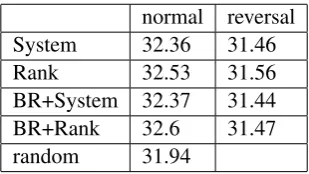
Table 4 lists the BLEU scores on the test set achieved by IncIHMM1 using different orders of hypotheses. The column ‘reversal’ shows the im-pact of deliberately bad order, viz. more than one BLEU point lower than the best order. The ran-dom order is a baseline for not caring about or-der of hypotheses at all, which is about 0.7 BLEU
normal reversal System 32.36 31.46
Rank 32.53 31.56
BR+System 32.37 31.44 BR+Rank 32.6 31.47 random 31.94
Table 4: Comparison between various orders of hypotheses. ‘System’ means system-based or-der; ‘Rank’ means N-best rank-based oror-der; ‘BR’ means Bayes Risk order of systems. The numbers are the BLEU scores on the test set.
point lower than the best order. Among the orders with good performance, it is observed that N-best rank order leads to about 0.2 to 0.3 BLEU point improvement, and that the Bayes Risk order of systems does not improve performance very much. In sum, the performance of incremental alignment is sensitive to the order of hypotheses, and the op-timal order is defined in terms of the rank of each hypothesis on some system’s n-best list.
8 Conclusions
This paper investigates the application of the in-cremental strategy to IHMM, one of the state-of-the-art alignment methods for MT output com-bination. Such a task is subject to the prob-lem of how to define state transitions on a grad-ually expanding CN. We proposed three differ-ent solutions, which share the principle that tran-sition over CN spans must be converted to the transition over word sequences provided by the component translations. While the consensus de-coding approach does not improve performance much, the two distortion models for incremental IHMM (IncIHMM1 and IncIHMM2) give superb performance in comparison with pair-wise TER, pair-wise IHMM, and incremental TER. We also showed that the order of hypotheses is important as a deliberately bad order would reduce transla-tion quality by one BLEU point.
References
Xiaodong He, Mei Yang, Jianfeng Gao, Patrick Nguyen, and Robert Moore 2008. Indirect-HMM-based Hypothesis Alignment for Combining
Out-puts from Machine Translation Systems.
Proceed-ings of EMNLP 2008.
System Combination using ITG-based Alignments. Proceedings of ACL 2008.
Evgeny Matusov, Nicola Ueffing and Hermann Ney. 2006. Computing Consensus Translation from Mul-tiple Machine Translation Systems using Enhanced
Hypothesis Alignment.Proceedings of EACL.
Nishanth Ulhas Nair and T.V. Sreenivas. 2007. Joint Decoding of Multiple Speech Patterns for Robust
Speech Recognition.Proceedings of ASRU.
Dennis Nilsson and Jacob Goldberger 2001. Sequen-tially Finding the N-Best List in Hidden Markov
Models.Proceedings of IJCAI 2001.
NIST 2008. The NIST Open Machine
Translation Evaluation. www.nist.gov/
speech/tests/mt/2008/doc/
Franz J. Och and Hermann Ney 2003. A Systematic Comparison of Various Statistical Alignment Mod-els. Computational Linguistics 29(1):pp 19-51
Kishore Papineni, Salim Roukos, Todd Ward and Wei-Jing Zhu 2002. BLEU: a Method for Automatic
Evaluation of Machine Translation. Proceedings of
ACL 2002
Antti-Veikko I. Rosti, Spyros Matsoukas, and Richard Schwartz 2007. Improved Word-level System
Com-bination for Machine Translation. Proceedings of
ACL 2007.
Antti-Veikko I. Rosti, Bing Zhang, Spyros Matsoukas, and Richard Schwartz 2008. Incremental Hypoth-esis Alignment for Building Confusion Networks with Application to Machine Translation System
Combination. Proceedings of the 3rd ACL
Work-shop on SMT.
Khe Chai Sim, William J. Byrne, Mark J.F. Gales, Hichem Sahbi, and Phil C. Woodland 2007. Con-sensus Network Decoding for Statistical Machine
Translation System Combination. Proceedings of
ICASSPvol. 4.
Matthew Snover, Bonnie Dorr, Rich Schwartz, Linnea Micciulla and John Makhoul 2006. A Study of Translation Edit Rate with Targeted Human