Online Full Text

(1)



Abstract— An analytical solution for non-orthogonal stagnation point for the steady flow of a viscous and incompressible fluid is presented. The governing nonlinear partial differential equations for the flow field are reduced to ordinary differential equations by using similarity transformations existed in the literature and are solved analytically by means of the Homotopy Analysis Method (HAM). The comparison of results from this paper and those published in the literature confirms the precise accuracy of the HAM. The resulting analytical equation from HAM is valid for entire physical domain and effective parameters.

Index Terms— Homotopy Analysis Method (HAM), Non-orthogonal, Stagnation flow, Stretching sheet, Analytical solution

I. INTRODUCTION

TAGNATION flow, fluid motion near the stagnation region, exists on all solid bodies moving in a fluid. Problems such as the extrusion of polymers in melt-spinning processes, glass blowing, the continuous casting of metals, and the spinning of fibers all involve some aspect of flow over a stretching sheet or cylindrical fiber [1].

Hiemenz was first to study two-dimensional stagnation flow using a similarity transform to reduce the Navier– Stokes equations to non-linear ordinary differential equation [2]. Chiam [3] studied stagnation point flow over stretching sheet. He considered various aspects of this problem such as normal or oblique two-dimensional and axisymmetric flows. Heat transfer of normal stagnation flow on a stretching sheet was later discussed by Mahapatra and Gupta [4]. Kimiaeifar et al. [5] investigated the steady flow of the third grade fluid in a porous half space. Kimiaeifar et al [6], studied two-dimensional stagnation flow towards a shrinking sheet. Recently, Lok et al. [7] modeled the stagnation flow

G.H. Bagheri is with the Department of Mechanical Engineering, Shahid Bahonar University of Kerman, Iran ([email protected]).

A. Kimiaefar is with the Department of Mechanical Engineering, Aalborg University, Pontoppidanstraede 101, DK-9220 Aalborg East, Denmark (corresponding author to provide phone: Tel/Fax: +4529293402; e-mail: ([email protected]).

A. Barari is with Department of Civil Engineering, Aalborg University, Aalborg, Denmark. ([email protected]).

A.R. Arabsolghar is with Department of Mechanical Engineering, Shahid Bahonar University of Kerman, Iran ([email protected]).

M. Rahimpour is with University of Applied Science and Technology, Kazeroon, Fars, Iran and National Elites Association, Teharn, Iran ([email protected]).

impinging on stretching sheet at some angle of incidence, by using numerical methods.

Analytical methods were used to study the viscous flow near a stagnation point. Xu et al. [8] studied the unsteady boundary layer flows of non-Newtonian fluids near a forward stagnation point. Hayat et al. [9], [10] investigated the MHD stagnation-point flow of an upper-convected Maxwell fluid over a stretching surface and MHD flow of a micropolar fluid near a stagnation-point towards a non-linear stretching surface. El-Ajou et al. [11] studied the construction of analytical solutions to fractional differential equations. Dommairy and N. Nadim [12] applied HAM and HPM in non–linear heat transfer equation. Fakhrai et al. [13] presented an analytical solution of BBMB equations. Recently Rahimpour et al. [14] studied the axisymmetric stagnation flow towards a shrinking sheet.

Nonlinear equations arose in many scientific problems and it is a challenging area for the researchers who want to solve these equations. There are some analytical solutions for a few numbers of nonlinear equations which are not applicable to the real world situations. Therefore, the only way to solving such nonlinear equations is numerical methods which among them we can address perturbation methods [15]. Stability and convergence are one of the most important issues with the numerical methods which should be taken into account to avoid divergence or inappropriate results. In the perturbation method, a small parameter is inserted in the equation and finding this small parameter and exerting it into the equations are deficiencies of this method. One of the semi-exact methods which does not need small/large parameters is the Homotopy Analysis Method (HAM), first proposed by Liao in 1992 [16], [17]. In this method the convergence region can be adjusted and controlled by an auxiliary parameter which is one of the important advantages of this method compare to other perturbation methods. It should be emphasized that the Homotopy Perturbation Method (HPM), introduced in 1998, is only a special case of HAM [18]–[21].

Up to now, no investigation has been made which provides an analytical solution for the non-orthogonal stagnation flow towards a stretching sheet. In this study, HAM is applied to find an analytical solution of nonlinear ordinary differential equations arising from the similarity solution, and the results were compared with those obtained in [7].

On the Analytical Solution of Non-Orthogonal

Stagnation Point Flow towards a Stretching

Sheet

A. Kimiaeifar, G.H. Bagheri, A. Barari, A.R. Arabsolghar and M. Rahimpour

S

IAENG International Journal of Applied Mathematics, 41:2, IJAM_41_2_02

(2)

II. FORMULATIONS

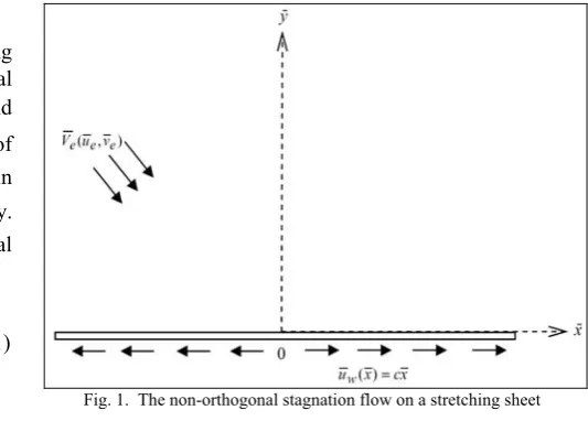
Considering stagnation point flow over a stretching surface in the x-axis direction in a two dimensional

Cartesian coordinate (x y, ). The fluid domain is y0 and

[image:2.595.285.552.49.240.2]

the flow with the velocity ( , )V u ve e e and different angle of incidence  impinges on the wall as shown schematically in Fig. 1, where ue and ve are velocity components at infinity. The governing equations for the steady two-dimensional incompressible flow are:

0,

u v

x y

 _ _

  (1)

2

1 _,

u u p

u v u

x y  x 

  

    

   (2)

2

1

,

v v p

u v v

x y  y 

 _  _{ }  _{ }

   (3)

where u and v are the velocity components along the x

and y directions, respectively,  is the density, p is the

pressure and



is the fluid kinematic viscosity. Considering no Slip wall boundary condition on the wall,

, 0, 0,

w w

u cx v  at y (4)

where c is the stretching rate. Velocity components at

infinity are as follow:

( sin ) ( cos ) ,

e

u  a  x b  y (5)

( sin ) , ,

e

v   a  y at y  (6)

where a and b are positive constants and  is a positive

parameter. It is worth mentioning that the external flow is a combination of a linear shear flow (shear stress b) parallel to the stream wise direction and a potential stagnation flow characterized by the constant a. Given the similarity transforms from [7]:

0.5 0.5

( )c , ( )c , .

x x y y  

  

   (7)

Near the stretching surface the scaled stream function is assumed in the form:

( ) ( ).

x f y g y

[image:2.595.278.552.57.430.2]

   (8)

Fig. 1. The non-orthogonal stagnation flow on a stretching sheet

Finally the Navier–Stokes equations are reduced to:

2 2_sin2 _0,

f ff f    (9)

cos 0,

g fg f g k   (10)

where  a c and kb c are positive constants. The

boundary conditions are defined as:

(0) 0, (0) 1, ( ) sin ,

f  f  f   (11)

(0)

(0) 0,

( )

cos ,

g



g





g



 

k



(12)

also f( ) ysin  and ( )g  ykcos can be

obtained, where



is a real constant and could be obtained by solving Eq. (9). By using ( )g y kh y( ) cos, Eq. (10) reduces to [7]:

0.

hfh f h   (13)

The boundary conditions for above equation are: (0) (0) 0, ( ) 1.

h h  h  (14)

The dimensionless skin friction is [7]:

2 2

0

(0) cos (0) . w

y

xf k h

y 

 

 _ 

 

 _ _   

  (15)

The location of the stagnation point, xs, is the place that the scaled streamlines  0 and the curve u0cross the wall at the stagnation point where w approaches zero, thus:

. ) 0 (

) 0 ( cos

f h k

xs _

 





(16)

IAENG International Journal of Applied Mathematics, 41:2, IJAM_41_2_02

(3)

III. APPLICATIONS

The governing equations for the non-orthogonal stagnation point flow towards a stretching sheet are expressed by Eq. (9) and Eq. (13). Nonlinear operators are defined as: 3 2 3 2 2 2 2 ( , ) ( , ) [ ( , )] ( , )

( , ) _{sin ( )} f

f y q f y q

N f y q f y q

y y

f y q

y  

        _ _     (17) 3 2 3 2 ( , ) ( , ) [ ( , )] ( , ) ( , ) ( , ) h

h y q h y q

N h y q f y q

y y

h y q f y q

y y 

            (18)

where q[0,1] is the embedding parameter and it should be

mentioned that the embedding parameter increases from 0 to 1, U y q( , ) and Y y q( , ) vary from the initial guess, U₀( )y

and Y y₀( ), to the exact solution, ( )U y and ( )Y y therefore it

is obtained: ), ( ) 1 , ( , ) ( ) 0 ,

(y U₀ y f y U y

f   (19)

). ( ) 1 , ( , ) ( ) 0 ,

(y Y₀ y h y Y y

h   (20)

Expanding f y q( , ) and h y q( , ) in Taylor series with

respect to q leads to:

, ) ( ) ( ) , ( 1 0



    m m m y q

U y

U q y

f (21)

, ) ( ) ( ) , ( 1 0



    m m m y q

Y y

Y q y

h (22)

where , ) , ( ! 1 ) ( 0     q m m m q q y f m y

U (23)

. ) , ( ! 1 ) ( 0     q m m m q q y h m y

Y (24)

Homotopy analysis method can be expressed by many different base functions [16]; according to the governing equations, it is straightforward to use a base function in the form of: , ) ( 1 1



      m my p p

py e

b y

U (25)

, ) ( 1 1



      m my p p

py e

d y

Y (26)

that bp and

d

p are the coefficients should be determined. When the base function is selected, the auxiliary functions

( )

f

H y , H_h( )y , initial approximations U₀( )y , Y y₀( ) and

the auxiliary linear operators L_f and L_h must be chosen in

such a way that the corresponding high-order deformation equations have solutions with the functional form similar to the base functions. This method is known as the rule of solution expression [17].

The linear operators Lf and Lh are chosen as:

, ) , ( ) , ( )] , (

[ 3 ₃ 2 ₂

y q y f y q y f q y f Lf     

 (27)

3 3

( , )

[ ( , )] ,

h

f y q L h y q

y

 

 (28)

with the property:

1 2 3

[ y] 0,

f

L c c yc e  (29)

, 0 ] [ 2 6 5

4c yc y 

c

L_h (30)

where c1 to c6 are the integral constants. According to the

rule of solution expression and the initial conditions, the initial approximations, U₀ and Y₀ as well as the integral

constants, c1 to c6 are formed as:

0 1 2 3 3

2 1 3

( ) ,

sin( ) 1,

sin( ), ,

y

U y c c y c e

c

c c c

             (31) 2 0 4 5 6

4 5 6

( ) ,

0, 1 / 2.

Y y c c y c y

c c c

  

   (32)

The zeroth order deformation equation for ( )f y is:

0

(1 ) [ ( , ) ( )] ( ) [ ( , )], f

f f

q L f y q U y

q H y N f y q

  

 (33)

(0, ) 0, (0, ) 1, ( , ) sin( ). f q f q y f q

y  

  _      (34)

where 0is a nonzero auxiliary parameter and according

IAENG International Journal of Applied Mathematics, 41:2, IJAM_41_2_02

(4)

to the rule of solution expression and from Eq. (33), the auxiliary functionH_f( )y can be chosen as follows:

( ) p ry. f

H y  y e (35)

Differentiating Eq. (33), m times, with respect to the

embedding parameter q and then setting q0 in the final

expression and dividing it by m!, it is reduced to:

1

1 0 0 0

1 2 3

( ) ( )

,

m m m

y y y

y

f m m

y

U y U y

H y e R U dy dydy

c c y c e

 _       

  



 (36)

(0) 0, (0) 0, ( ) 0.

m m m

U  U  U   (37)

Eq. (36) is the mth_{order deformation equation for}

f y

( )

_, where: 2 2 1 1 3 2 1 1 3 2 0 1 1 0

( ) sin

( ) _{( )} ( )

( ) ( )

,

m m m

m

m m z

z z m m z z z R U

d U y d U y

U y dy dy dU y dU y dy dy                   _ _     _ _  



      (38) and 0, 1 . 1, 1 m m m  _{ }  

 (39)

The rate of convergence can be increased when suitable values are selected for r and p. According to the rule of

solution expression the suitable values for r and p are

{p0,r1}. Consequently, the corresponding auxiliary function was determined as ( ) y

f

H y e . As a result of this

selection, the solution’s series ( )U y , is developed up to

18th order of approximation, so ( )f y is obtained as

follows: 18 0 1 0 2 2

2 2 2

2 2 2 2 2

( ) ( ) ( ) ( )

1 sin( ) sin( )

1

( sin( ) 1) (2sin( )

4

2 2 cos ( ) 5 sin( )

5 5 cos ( )

3 sin( ) sin( ) 3

3 cos ( )

cos ( )) .

m m

y

y y

y y y

y y

y

f y U y U y U y

y

e

e e

e e e

e e y

y e                                                        



   (40)

The zeroth order deformation equation for h y( ) is:

0

(1 ) [ ( , ) ( )]

( ) [ ( , )],

h

h h

q L h y q Y y

q H y N h y q

  

 (41)

2 2

(0, ) 0, h(0, ) 0, h( , ) 1.

h q q q

y y

 

   

  (42)

Auxiliary function and mth_{order deformation equation for} 1

m are: ( ) 1,

h

H y  (43)

1

1 0 0 0

2 4 5 6

( ) ( )

,

m m m

y y y

h m m

Y y Y y

H y R Y dy dy dy

c c y c y

 _



 

  

  



 (44)

(0) 0, ( ) 0.

m m m

Y Y  Y   (45)

Since f and h are coupled in Eq. (13), the order of approximation for f y( ) in this equation is limited to 8.

Eq. (44) is the mth_{order deformation equation for}_{h y}_{( )}_, where:

3 2

1 1

1 ₃ ₂

1 ( ) ( ) ( ) ( ) ( ) ( ) _, m m m m m m

d Y y d Y y

R Y f y

dy d y

dY y df y

dy dy  

        _ _     

 (46)

and . 1 , 1 1 , 0       m m m



(47)

By developing the solution’s series, ( )Y y , up to 10th

order of approximation, ( )h y is obtained:

10

2 0 1

0

2 5 2 2 5 6 2 2 10 12 2

10 12 6

1

( ) ( ) ( ) ( )

2 0.3743967885 sin( )cos ( ) 4.820986454 10 cos ( ) 3.647607224 10

3.647607224 10 .

m m y y y y

h y Y y Y y Y y y

e y e y e e                            



      (48)

IAENG International Journal of Applied Mathematics, 41:2, IJAM_41_2_02

(5)

IV. CONVERGENCE OF HAM SOLUTION

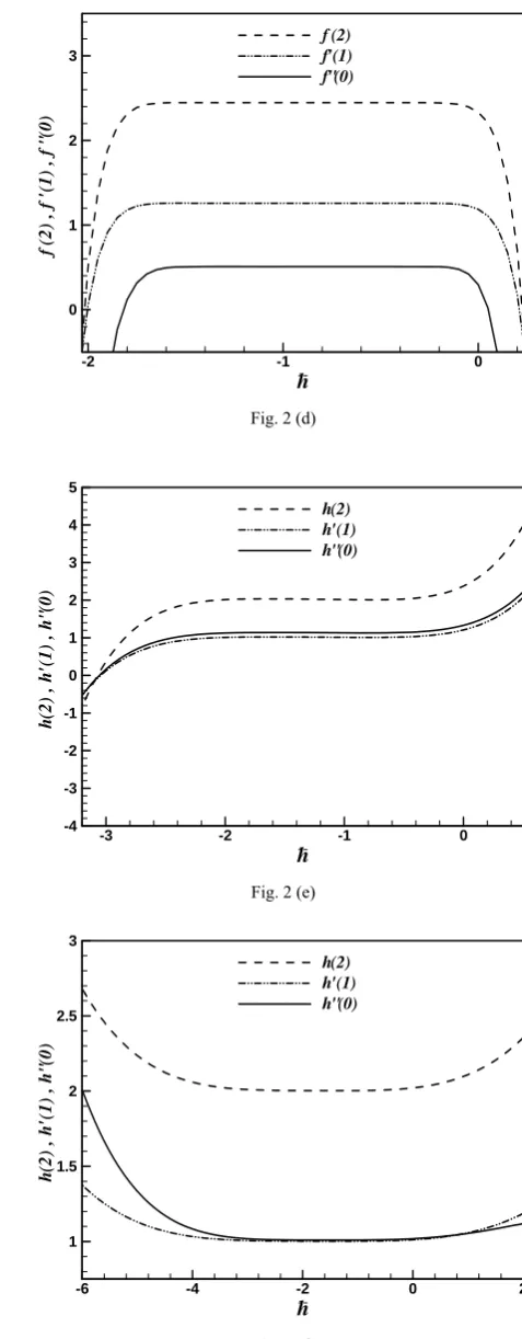
The analytical solution should converge. The convergence and accuracy of the solution series should be controlled, therefore it should be noted that the auxiliary parameter , as pointed out by Liao [17]. In order to define a region where the solution series is independent on , a multiple of -curves are plotted. The region where the distribution of f, f, f and h, h, h versus  is a horizontal line is known as the convergence region for the corresponding function. The common region among the f

and its derivatives,

h

and its derivative are known as the overall convergence region.

To study the influence of  on the convergence of solution, the -curve of f(0), f(1), f(2)and h(0),

(1)

h , (2)h are plotted respectively by 18th order and 10th

order approximation of solution for some selected  and  , as shown in Fig. 2. Furthermore, increasing the order of approximation decreases the relative error, as shown in Fig. 3.

V. RESULTS AND DISCUSSION

After solving equations (9) and (13) with the boundary conditions described in equations (11) and (14) with the HAM for different values of



and



the following results obtained. Calculated values of f(0), and

x

_s are shown in Table 1, Table 2 and Table 3 for different values of  and , respectively. In these tables HAM results also are compared with the results of [7] and showed that HAM provides an analytical solution with high order of accuracy within a few numbers of iterations.

As it can be seen from Table 1 results show that f(0) has a strong nonlinear behavior respect to but increasing

 lead to increscent of f(0). Unlike f(0),  varies in a

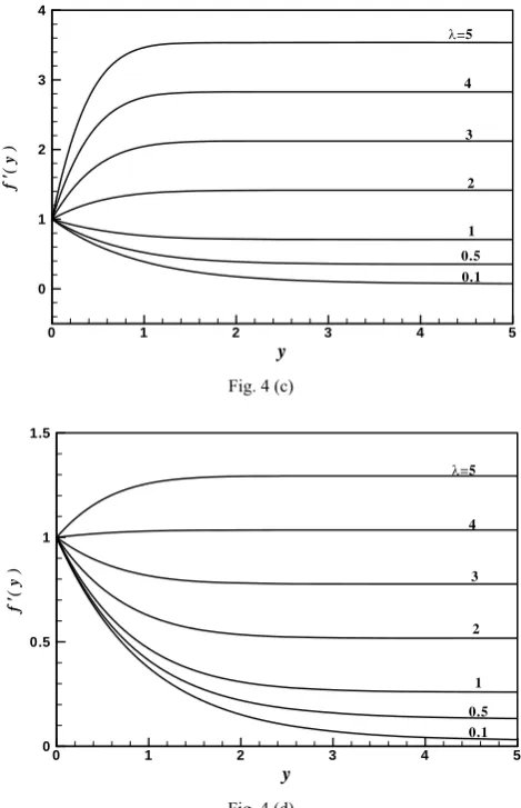
linear manner respect to  and  as it is presented in Table 2. Based on this table we can see that  decreases when values of  and increased. Results in the Table 3 show that xs has a nonlinear variation respect to  and . In the Fig. 4 variation of f respect to yis presented for different

values of and  .

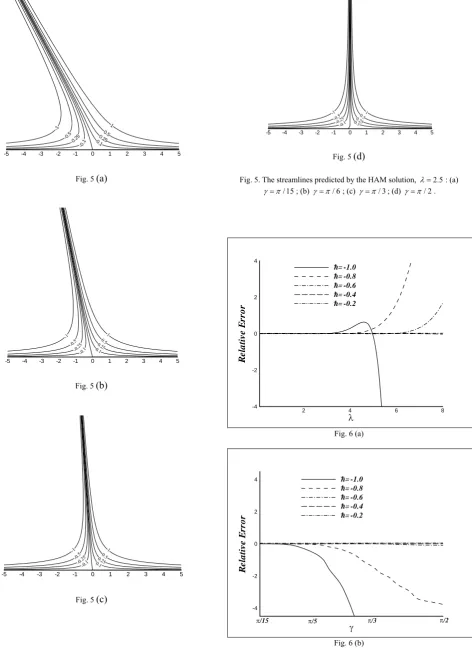
According to this figure it can be seen when  increases, the boundary layer thickness decreases, as it is observed in [7]. The effects of  and  on scaled streamlines are shown in Fig. 5. As mentioned before, HAM can provide an analytical solution which is acceptable for all values of y and other effective parameter such as  and . Eq. (49) presents an expression for ( , , )f y  with 10 orders of

approximation:

2 2 2 2 2 2

2 2 3

3 2 2 3

2 2 2 2 3

( ) sin( ) 0.3 0.3 sin ( ) 1.9058333 sin ( ) 0.2246296 cos ( )

0.8 sin ( ) 0.1188 sin( ) 0.11879629 sin( ) cos ( ) 8.59259 10 sin( )

0.2 sin ( ) 0.21 sin( ) 0.4

y

y y

y

y y

f y

e

e e

e

e e

    

 

   

  

 

   



 



 

    

 

 



 

 

2

3 4 2 2 2 4 2 2

3 4 3

sin( )

6.6667 10 cos ( ) 1.05556 10 cos ( ) 5.277778 10 sin( ) ...

y

ye

e

 



 



 

 

(49)

Note that, as pointed in [18]–[20], the results given by the “Homotopy Perturbation Method” are exactly the same as those given by the HAM when  1 and ( ) 1H  ,

because the “Homotopy Perturbation Method” is only a special case of the HAM. The comparison between HAM and HPM for f(0) is shown in Fig. 6. The figure shows that for 3 and   / 6, the prediction of two methods are identical, and when  and  increase (3 and

/ 6

  ); the deviation between two methods becomes more significant, because the HPM solution gets divergent.

VI. CONCLUSIONS

The nonlinear differential equations resulting from similarity solution of non-orthogonal stagnation point flow towards a stretching sheet is studied using the Homotopy Analysis Method. The comparison with numerical results and convergence study shows that using approximations of small orders, results in satisfactory accuracy and increasing the order of approximation, the accuracy increases. After demonstrating the effectiveness of HAM, as a powerful analytical technique, the effects of different parameters such as  and on the velocity distribution are presented.

The proposed analytical approach has many applications, and thus may be applied in similar ways to other boundary-layer flows to obtain accurate series solutions.

IAENG International Journal of Applied Mathematics, 41:2, IJAM_41_2_02

(6)

h

f

(2)

,

f

'(

1)

,

f

"(

0

)

-2 -1 0

-1 0 1 2

f (2) f'(1) f"(0)

--Fig. 2 (a)

h

f

(2)

,

f

'(

1)

,

f

"(

0

)

-2 -1 0

-1 0 1 2 3

f (2) f'(1) f"(0)

--Fig. 2 (b)

h

f

(2)

,

f

'(

1)

,

f

"(

0

)

-1 0

1 2 3 4 5

f (2) f'(1) f"(0)

--Fig. 2 (c)

h

f

(2)

,

f

'(

1)

,

f

"(

0

)

-2 -1 0

0 1 2 3

f (2) f'(1) f"(0)

--Fig. 2 (d)

h

(2)

,

h

'(

1

)

,

h

"(

0)

-3 -2 -1 0

-4 -3 -2 -1 0 1 2 3 4 5

h(2) h'(1) h"(0)

--Fig. 2 (e)

h

(2)

,

h

'(

1

)

,

h

"(

0)

-6 -4 -2 0 2

1 1.5 2 2.5 3

h(2) h'(1) h"(0)

--Fig. 2 (f)

Fig. 2. The -curves to indicate the convergence region: (a) 0.1, / 2

  ; (b) 1.0,   / 3; (c) 3.0,   / 4; (d) 5.0, / 12

  ; (e) 2.5,   / 4; (f) 4.0,   / 12.

[image:6.595.64.476.46.680.2] [image:6.595.53.285.56.735.2] [image:6.595.297.536.62.674.2]

(7)

Order of series solution

Re

la

ti

v

e

Er

ro

r

5 10

-0.1 0 0.1 0.2 0.3 0.4 0.5

=/3,= 0.5

=/12,= 1

=/2,= 2

=/4,= 3

Fig. 3. The effect of order of approximation on Relative Error. (Relative error define as



f(0)Numericf(0)HAM



f(0)Numeric ).

y

f'

(

y

)

0 1 2 3 4 5

0 1 2 3 4 5 6

0.1 =5

4

3

2

1

0.5

Fig. 4 (a)

y

f'

(

y

)

0 1 2 3 4 5

0.1

=5

4

3

2

1 0.5

Fig. 4 (b)

y

f'

(

y

)

0 1 2 3 4 5

0 1 2 3 4

0.1

=5

4

3

2

1 0.5

Fig. 4 (c)

y

f'

(

y

)

0 1 2 3 4 5

0 0.5 1 1.5

0.1

=5

4

3

2

1

0.5

Fig. 4 (d)

Fig. 4. Functionf( )y , predicted by the HAM solution: (a)   / 2; (b)   / 3; (c)   / 4; (d)   /12

IAENG International Journal of Applied Mathematics, 41:2, IJAM_41_2_02

(8)

-1

-0.5

-0.2 5

-0.1 0.1 0.20.5₅

1

-5 -4 -3 -2 -1 0 1 2 3 4 5

Fig. 5 (a)

-1 -0.5

-0.25_-0.1 0.10.25 0.51

-5 -4 -3 -2 -1 0 1 2 3 4 5

Fig. 5 (b)

-1

-0.5

-0.25 -0.1 0.10.25

0.51

-5 -4 -3 -2 -1 0 1 2 3 4 5

Fig. 5 (c)

-1 -0.5

-0.25 -0.1 0.10.25

0.51

-5 -4 -3 -2 -1 0 1 2 3 4 5

Fig. 5 (d)

Fig. 5. The streamlines predicted by the HAM solution, 2.5: (a) / 15

  ; (b)   / 6; (c)   / 3; (d)   / 2.



R

e

la

tiv

e

E

rr

o

r

2 4 6 8

-4 -2 0 2 4

h= -1.0 h= -0.8 h= -0.6 h= -0.4 h= -0.2

Fig. 6 (a)



R

e

la

tiv

e

E

rr

o

r

-4 -2 0 2

4 h= -1.0 h= -0.8 h= -0.6 h= -0.4 h= -0.2

/15 /5 /3 /2

Fig. 6 (b)

Fig. 6. Relative Error of 18th order HAM solution: (a)   / 4; (b) 5. Relative Error is defined as



f(0)_Numericf(0)_HAM



f(0)_Numeric ).

(9)

TABLEI

COMPARING THE PRESENT ANALYTICAL AND NUMERICAL RESULTS FORf(0) WITH THE NUMERICAL RESULTS OF [7],[4] AND [5]

 f(0)

15 / 

 12/ /6 /4 /3 /2

Present [7] [4] [5]

0.1 -0.995598 -0.994472 -0.987580 -0.980613 -0.933641 -0.969336 -0.969388 -0.969400 -0.969400 -0.994348* _-0.980700*_-0.933660*

0.5 -0.967722 -0.956475 -0.885797 -0.806194 -0.734437 -0.667275 -0.667271 -0.667300 -0.667300 -0.956268*_-0.806205*_-0.734444*

1 -0.913276 -0.879695 -0.667264 -0.424228 -0.205018 — — — — -0.879674*_-0.424315*_-0.205025*

2 -0.750707 -0.648648 0.000000 0.738433 1.400960 2.017491 2.017615 2.017500 2.017500 -0.648613*_0.738474*_1.401023*

3 -0.528237 -0.331944 0.909530 2.313073 3.566574 4.729456 4.729694 4.729300 4.729600 -0.331937*_2.313144*_3.566614*

4 -0.254722 0.056877 2.017503 4.221816 6.184068 8.001139 8.001379 — — 0.056886*_4.221839*_6.184095*

5 0.063870 0.508974 3.296959 6.418007 9.187889 11.751991 11.753760 — — 0.508995*_6.418018*_9.189975*

THE SUPERSCRIPT * IS FROM [7]

TABLEII

VARIATIONS OF  WITH RESPECT TO  AND 

 

/15

    /12   / 6   / 4   / 3   / 2

0.1 0.948837 0.937121 0.885257 0.844550 0.815224 0.791705 0.948840* _0.937146*_0.885260*_0.844538*_0.815253*

0.5 0.784950 0.743188 0.577234 0.462835 0.386766 0.328594 0.784941*_0.743196*_0.577249*_0.462841*_0.386747*

1 0.630245 0.566690 0.328612 0.174330 0.074789 — 0.630258*_0.566681*_0.328601*_0.174313*_0.074780*

2 0.402481 0.314049 — -0.194558 -0.318151 -0.410406 0.402497*_0.314069*_{— -0.194572}*_-0.318141*

3 0.232485 0.129225 -0.229744 -0.449356 -0.588801 -0.693056 0.232477*_0.129230*_-0.229705*_-0.449360*_-0.588790*

4 0.095224 -0.018534 -0.410433 -0.649838 -0.802213 -0.916502 0.095215*_-0.018542*_-0.410425*_-0.649826*_-0.802232*

5 -0.020777 -0.142647 -0.561671 -0.818124 -0.981979 -1.105170 -0.02076*_-0.142771*_-0.56166*_-0.818131*_-0.981994*

TABLEIII

VARIATIONS OF THE LOCATION OF STAGNATION POINT, x_s, WITH RESPECT TO  AND 

 xs

 /15  /12  /6  /4  /3

0.1 -0.024495 0.013777 0.096788 0.129686 0.116341 0.013796* _0.096778*_0.129673*_0.116440*

0.5 -0.734288 0.337793 0.531590 0.581741 0.499358 0.337787*_0.531582*_0.581737*_0.499344*

1 1.326771 0.610011 1.015793 1.493927 2.337632 0.609998*_1.015784*_1.493930*_2.337573*

2 0.937517 1.183010 — -1.043772 -0.405385 1.183009*_—_-1.043765*_-0.405374*

3 1.585532 2.693435 -1.051013 -0.359658 -0.169953 2.693444*_-1.051062*_-0.359664*_-0.169948*

4 3.634407 -17.143788 -0.500180 -0.205309 -0.101474 -17.143792*_-0.500169*_-0.205311*_-0.101470*

5 -15.479858 -2.027413 -0.316717 -0.138553 -0.069771 -2.027498*_-0.31673*_-0.138567*_-0.069767*

IAENG International Journal of Applied Mathematics, 41:2, IJAM_41_2_02

(10)

REFERENCES

[1] J. Paullet and P. Weidman, “Analysis of stagnation point flow toward a stretching sheet,” International Journal of Non-Linear Mechanics, vol. 42, pp.1084–1091, 2007.

[2] K. Hiemenz, “Die Grenzschicht an einem in den gleichformingen Flussigkeitsstrom eingetauchten graden Kreiszylinder,” Dinglers Polytechnic Journal, vol. 326, pp. 321–324, 1911.

[3] T.C. Chiam, “Stagnation-point flow towards a stretching plate,”

Journal of Physical Society of Japan, vol. 63, pp. 2443–2444, 1994. [4] T.R. Mahapatra and A.S Gupta, “Heat transfer in stagnation-point

flow towards a stretching sheet,” Journal of Heat and Mass Transfer, vol. 38, pp. 517–521, 2002.

[5] A. Kimiaeifar, O.T. Thomsen and E. Lund, “Assessment of HPM with HAM to find an analytical solution for the steady flow of the third grade fluid in a porous half space,” IMA Journal of Applied Mathematics, pp.1−14, 2010.

[6] A. Kimiaeifar, G.H. Bagheri, M. Rahimpour and M.A. Mehrabian, “Analytical Solution of Two-Dimensional Stagnation Flow towards a Shrinking Sheet by Means of Homotopy Analysis Method”, Journal of Process Mechanical Engineering, vol. 223, pp. 133-143, 2009.

[7] Y.Y. Lok, N. Amin, and I. Pop, “Non-orthogonal stagnation point flow towards a stretching sheet,” International Journal of Non-Linear Mechanics, vol. 41, pp. 622–627, 2006.

[8] H. Xu, S.J. Liao, and I. Pop, “Series solution of unsteady boundary layer flows of non-Newtonian fluids near a forward stagnation point,”

Journal of Non-Newtonian Fluid Mechanics, vol. 139, pp. 31–43, 2006.

[9] T. Hayat, Z. Abbas and M. Sajid, “MHD stagnation-point flow of an upper-convected Maxwell fluid over a stretching surface,” Chaos, Solitons & Fractals, vol. 39, pp. 840–848, 2009.

[10] T. Hayat, T. Javed and Z. Abbas, “MHD flow of a micropolar fluid near a stagnation-point towards a non-linear stretching surface,” Nonlinear Analysis: Real World Applications, vol. 10, pp. 1514– 1526, 2009.

[11] Ahmad El-Ajou, Zaid Odibat, Shaher Momani, Ahmad Alawneh, Construction of analytical solutions to fractional differential equations using homotopy analysis method, IAENG International Journal of Applied Mathematics, 40:2, IJAM_40_2_01.

[12] G. Domairry and N. Nadim, “Assessment of homotopy analysis method and homotopy Perturbation method in non–linear heat transfer equation,” International Communications in Heat and Mass Transfer, vol. 35, pp. 93–102, 2008.

[13] A. Fakhari, G. Domairry and Ebrahimpour, “Approximate explicit solutions of nonlinear BBMB equations by homotopy analysis method and comparison with the exact solution,” Physics Letters A, vol. 368,

pp. 64–68, 2007.

[14] M. Rahimpour, S.R. Mohebpour, A. Kimiaeifar, and G.H. Bagheri, “On the analytical solution of axisymmetric stagnation flow towards a shrinking sheet,” International journal of mechanics, vol. 2, pp. 1-10, 2008.

[15] A.H. Nayfeh, Problems in Perturbation. Second edition, NY: John Wiley & Sons, 1993.

[16] S.J. Liao, “The proposed homotopy analysis technique for the solution of nonlinear problems,” Ph.D. thesis, Shanghai Jiao Tong University, 1992.

[17] S.J. Liao, Beyond perturbation: introduction to the homotopy analysis method, Boca Raton: Chapman &Hall/CRC Press, 2003.

[18] S.J. Liao, “Comparison between the homotopy analysis method and homotopy perturbation method,” Applied Mathematics and Computation, vol. 169, pp. 1186–1194, 2005.

[19] A. Kimiaeifar, “An analytical approach to investigate the response and stability of Van der Pol-Mathieu-Duffing oscillators under different excitation functions,” Journal of Mathematical Methods in the Applied Sciences, vol. 33, pp. 1571–1577, 2010.

[20] A. Kimiaeifar, A.R. Saidi, G.H. Bagheri, M. Rahimpour and D.G Domairry, “Analytical solution for Van der Pol –Duffing oscillators,”

Chaos, Solitons and Fractals, vol. 42, pp. 2660–2666, 2009.

[21] Mo. Rokibul Islam and M. Ali Akbar, A New Asymptotic Solution for Third Order More Critically Damped Nonlinear Systems, IAENG International Journal of Applied Mathematics, 39:1, pp9-pp15.