Predicting Credit Card Transaction Fraud Using Machine Learning Algorithms

(1)

ISSN Print: 2150-8402

DOI: 10.4236/jilsa.2019.113003 Aug. 14, 2019 33 Journal of Intelligent Learning Systems and Applications

Predicting Credit Card Transaction Fraud Using

Machine Learning Algorithms

Jiaxin Gao

1

, Zirui Zhou

2*

, Jiangshan Ai

3

, Bingxin Xia

4

, Stephen Coggeshall

5

1_{Hebei University of Economics and Business, Shijiazhuang, China}

2_{China University of Political Science and Law, Beijing, China}

3_{Wuhan Maple Leaf International School (High School), Wuhan, China}

4_{Wuhan Jinde Education Consulting, Co., Ltd., Wuhan, China}

5_{University of Southern California, Los Angeles, USA}

Abstract

Credit card fraud is a wide-ranging issue for financial institutions, involving theft and fraud committed using a payment card. In this paper, we explore the application of linear and nonlinear statistical modeling and machine learning models on real credit card transaction data. The models built are supervised fraud models that attempt to identify which transactions are most likely fraudulent. We discuss the processes of data exploration, data cleaning, variable creation, feature selection, model algorithms, and results. Five different supervised models are explored and compared including lo-gistic regression, neural networks, random forest, boosted tree and support vector machines. The boosted tree model shows the best fraud detection re-sult (FDR = 49.83%) for this particular data set. The rere-sulting model can be utilized in a credit card fraud detection system. A similar model development process can be performed in related business domains such as insurance and telecommunications, to avoid or detect fraudulent activity.

Keywords

Credit Card Fraud, Machine Learning Algorithms, Logistic Regression, Neural Networks, Random Forest, Boosted Tree, Support Vector Machines

1. Introduction

Credit card fraud remains an important issue for theft and fraud committed us-ing a payment card, such as a credit card or debit card. To combat this many fraud detection algorithms are widely used in industry [1] [2] [3] [4]. Card fraud can happen with the theft of the physical card as well as with the compromise of

How to cite this paper: Gao, J.X., Zhou, Z.R., Ai, J.S., Xia, B.X. and Coggeshall, S. (2019) Predicting Credit Card Transaction Fraud Using Machine Learning Algorithms. Journal of Intelligent Learning Systems and Applications, 11, 33-63.

https://doi.org/10.4236/jilsa.2019.113003

Received: April 6, 2019 Accepted: August 11, 2019 Published: August 14, 2019

(2)

DOI: 10.4236/jilsa.2019.113003 34 Journal of Intelligent Learning Systems and Applications

the card, including skimming, breach, account takeover, that would otherwise look like a legitimate transaction. According to the Global Payments Report 2015 [5], the credit card is the highest-used payment method globally in 2014 compared to other methods such as an e-wallet and Bank Transfer. Along with the rise of credit card usage, the number of fraud cases has also been steadily in-creasing [6]. The rise in credit card fraud has a large impact on the financial in-dustry. The global credit card fraud in 2015 reached a staggering USD 21.84 bil-lion [7].

Financial institutions today typically develop custom fraud detection systems targeted to their own portfolios [8]. The data mining and machine learning techniques are vastly embraced to analyze patterns of normal and unusual beha-vior as well as individual transactions in order to flag likely fraud. Given the re-ality, the best cost-effective option is to tease out possible evidence of fraud from the available data using statistical algorithms [9]. Supervised models trained on labeled data examine all previous labeled transactions to mathematically deter-mine how a typical fraudulent transaction looks and assigns a fraud probability score to each transaction [10]. Among the supervised algorithms typically used, the neural network is popular, and support vector machines (SVMs) have been applied, as well as decision trees and other models [3] [9] [11]-[21]. However, little attention has been devoted in the literature to some comparison of all the common algorithms, particularly using real data sets.

In this paper, we explore the application of various linear and nonlinear statis-tical modeling and machine learning models on credit card transaction data. The models built are supervised fraud models that attempt to identify which transac-tions are most likely fraudulent.

2. Description of Data

The data available for this research project are a collection of credit card transac-tions from a government agency located in Tennessee, U.S.A. The particular agency is not known.

The data consist of 96,753 credit card transactions during the year 2010, with 1059 labeled as fraud. The file contains the fields:

• _{Record: A unique identifier for each data record. This field also represents}

the time order;

• _{Cardnum: The account number for the transactions (we note that they are}

Mastercard transaction since the account numbers begin with the digits 54);

• _{Date: The date of the transaction. Month, day and year only (no time of day);} • _{Merchnum: A typically 12-digit merchant identification number;}

• _{Merch Description: A brief text description field of the merchant, typically}

around 20 characters;

• _{Merch State: The state of the address for the merchant;} • _{Merch Zip: The zip code of the merchant;}

(3)

DOI: 10.4236/jilsa.2019.113003 35 Journal of Intelligent Learning Systems and Applications • _{Amount: The dollar amount of the transaction;}

• _{Fraud: A label for the transaction to indicate whether or not it was a}

[image:3.595.59.542.461.712.2]

fraudu-lent transaction.

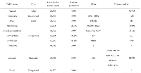
Table 1 shows summary information about all the fields. Only the Amount field is a numeric type field; the other fields are all categorical or text. The statis-tical magnitudes in the table were calculated with the outliers eliminated. Three fields have some missing values: Merchnum, Merch state, and Merch zip. It was noticed that the number of unique values of the Merch state field is 227, which is unexpected because the U.S. has only 50 states. Some of the values in this field might be from other countries, such as Canada and/or Mexico.

Below we show some further information about the data.

Figure 1 shows the number of transactions each month. We noticed the gen-eral upward trend through September, followed by a sharp drop in October. The monthly transactions are fewer in the last quarter of the year compared with other quarters. This is due to the government fiscal year which starts on October 1, and people tend to be more cautious with their money in the first few months of the new fiscal year.

Figure 2 shows the top 10 of the most frequently traded merchant descrip-tions. The total transaction frequency of the top 15 categories is 13,256, which is about 13.7% of the records. The top 200 categories account for 41% of the total records. In Table 1, we see that there are 13,126 kinds of merchants by this Merch description field, and 48.6% of the merchant descriptions only occurred once.

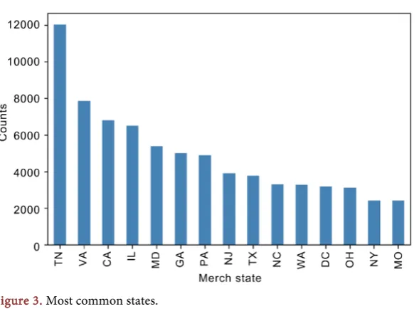
Figure 3 depicts the top 10 of the most frequently observed merchant states.

Table 1. Summary description of the data set.

Fields name Type Records that _{have a value} _populatedPercent Mode # Unique values

Record Index 96,753 100% 96,753

Cardnum Categorical 96,753 100% 5142148452 1645

Date Time 96,753 100% 2/28/10 365

Merchnum

Categorical

93,378 96.5% 930090121224 13,091

Merch description 96,753 100% GSA-FSS-ADV 13,126

Merch state 95,558 98.8% TN 227

Merch zip 92,097 95.2% 38118 4567

Transtype 96,753 100% P 4

Amount Numeric 96,753 100% 3.62

Mean 395.33*

34,909 Max 30372.46*

Min 0.01 Std 814.74*

Fraud Categorical 96,753 100% 0 2

(4)

[image:4.595.227.528.66.258.2] [image:4.595.228.518.289.483.2]

DOI: 10.4236/jilsa.2019.113003 36 Journal of Intelligent Learning Systems and Applications Figure 1. Monthly count of transactions shows seasonality.

Figure 2. Most common merchant descriptions.

[image:4.595.229.524.509.726.2]

(5)

The most frequent state is TN which is about 12.6% of the whole transaction frequency, and is not surprising because that is where the facility is located. The total number of transactions in the top 15 states is 71,647, which is about 75% of the entire records. From Table 1 we see that there are 227 different states in the data. And we note that 168 of the state’s field values are numbers rather than letters.

3. Data Cleaning

[image:5.595.209.545.367.604.2]

When we examine the field Amount, shown in the box plot distribution Figure 4, we see that there is one large outlier with the Amount value recorded as over 3 million dollars. After thoroughly checking that particular record, which is not labeled as fraud, we discover that it is an unusual but known transaction in Mexican pesos from a particular Mexican organization, and we thus exclude it from further analysis.

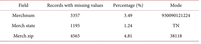
Table 2 shows the information about the fields with missing values. All of these three fields have a strong relationship with the field Merch description, but the same Merch description may also correspond to different values in the three above fields. These three fields also have a strong relationship with each other, so the mode of each field is used to fill in the missing fields.

[image:5.595.210.542.657.730.2]

Figure 4. Box plot distribution of the Amount field.

Table 2. Fields with missing values.

Field Records with missing values Percentage (%) Mode

Merchnum 3357 3.49 930090121224

Merch state 1195 1.24 TN

Merch zip 4565 4.81 38118

0 1.0e+06 2.0e+06 3.0e+06

(6)

4. Variable Creation

Creating expert variables is a critical step before any model can be built. We examine the original fields from the raw data set, as shown in Table 1, and from these we create a large universe of candidate variables for our supervised models. At this stage, we want to create as many candidate variables as possible, and later we will use a variety of feature selection methods to reduce the universe of can-didate variables to those that will be our final set of possible model inputs.

This step of creating variables, also called feature engineering, requires us to know as much as possible about the dynamics of the particular problem we are trying to solve. We want to do our best to create variables that in themselves contain as much encapsulated information of the signals of anomalous behavior that could be fraud. Thus we interview domain experts to fully understand as best as possible the different modes of fraud for this problem and try to build va-riables that will show the signals of these fraud modes.

This step of variable creation is arguably the most important step in machine learning. Encapsulating the problem dynamics as best as possible into these ex-pert variables, prepares the data for the model in an as optimal way as possible. One should always do as much work upfront in this stage as possible in order to minimize the work required by your machine learning algorithm. It is true that theoretically all these nonlinear algorithms can discover these expert variable dynamics themselves, but it is generally difficult in a high dimensional space with sparse data sets. We note that 100,000 records are sparse data in anything above a handful of dimensions. Thus we work hard to create a universe of can-didate variables that have encoded in them as best as possible as many indicators of potential fraud as we can think of. The logic behind these special expert va-riables is described below [22].

There are four general types of expert variables that have been built:

1) Amount variables. These variables are important because the amount spent can be immediately indicative of unusual activity. For example, if a person typi-cally spends about 400 dollars over some time window and one day he spends 400,000 dollars in one transaction, it would be a signal of odd behavior. There-fore these amount-type variables are good candidates to detect potential frauds.

maximum median

total cardnum

actual-average merchnum

amount spent by at this

actual-median cardnum on this merchnum

actual average cardnum in this zip code

actual max cardnum in

actual total actual median              1 day 7 days over the last

14 days 30 days this state            _ 

(7)

that if a person does 2 transactions per day usually, but one day he does 2000 transactions. That will be suspicious. So frequency variables are helpful to see if there is a big difference in a number of transactions.

cardnum merchnum

number of transactions with same cardnum and merchnum cardnum and zip code cardnum and state 1 day

7 days over the last

14 days 30 days             

3) Days since variables. One example is that if it has been 10 months since the last time a person uses his card, someone else might be using it in this case, so that it might be a fraud.

Current transaction date minus date of most recent transaction with same cardnum

merchnum

cardnum and merchnum cardnum and zip code cardnum and state

      

4) Velocity variables. This measure shows how a person may do a large num-ber of transactions over a day compared to his average transactions over a period of time. It is similar to the frequency variables.

cardnum

number of transactions with same over the last 1 day

merchnum

7 days cardnum

average daily number of transactions for this over the last 14 days

merchnum 30 days           

with some variations of characteristics we end up 200 variables of the first type, 20 variables of the second type, 5 variables of the third type and 12 variables of the fourth type. These 237 expert variables are listed in Appendix.

5. Feature Selection

(8)

carry the more useful information.

In general, there are three categories of feature selection methods: filter, wrapper, and embedded methods. The former two are applied in this research. A filter is a method applied to the data set without using a particular standard modeling algorithm. The wrapper method “wraps” a particular model around the feature selection process, for example, stepwise selection. Finally, an embed-ded method has the feature selection built directly into the modeling process, such as various tree methods or the use of regularization.

Here we first apply a filter method of feature selection to reduce the number of variables by about half. By calculating certain performance measures across every single variable individually and ranking the variables by these measures, a filter method can efficiently identify those with low performance. The particular filter measures we use for this fraud problem are a univariate Kolmogo-rov-Smirnov (KS) and the univariate fraud detection rate (FDR) at 3%. The Kolmogorov-Smirnov statistical test is a measure to quantitatively determine how much two distributions over the same independent variable are separated. This is a common test used for feature selection in a binary classification prob-lem. Here we build the distribution of the two categories of records, one for each of the two dependent variables values, across each of the independent variables, one by one. The question we are asking is how well each independent variable by itself can differentiate the two classes. The equations for calculating the KS sepa-ration of two distributions are:

Kolmogorov-Smirnov Formula

min

max _xx _good _b_ad d

x

KS=

_∫

_P −P _ x

min

max go d

x od

x x

ba

KS=

∑

_P −P _

where the first representation is for a continuous distribution and the second is what we use in practice for finite data sets.

For each candidate variable, we build the two distributions of the frauds and the non-frauds by this variable, and we calculate the KS separation between these two distributions. This measure explicitly tells how well each candidate va-riable by itself can separate the classes, and is, in essence, a univariate model.

(9)

FDR (10% fraud at 3% penetration) is a measure of how well the candidate vari-able by itself separates the frauds from the non-frauds.

A wrapper is a popular feature selection method to help determine which va-riables should be included in the machine learning model. It directly builds many models with different sets of variables, selecting them by examining the measure of goodness of the model itself. The most common wrapper method is stepwise selec-tion, typically forward or backward selection. For forward selecselec-tion, we first build univariate models, one for each of the n candidate variables, and examine the measure of goodness for each model. We select the variable xi whose univariate

model is best and then proceed by building n-1 two-variable models, xi combined

with all the remaining candidate variables, one by one. We select the best 2-variable model, now having identified xi and another xj as the strongest variables

(xj strong in conjunction with xi). We continue this stepwise forward selection

un-til we see negligible improvement when adding a new variable.

Backward selection is similar. Here we start with a single n-variable mode that uses all candidate variables. We then build n new models, each using only n-1 variables, where we have removed one of the n possible variables from each new model. The variable whose n-1 model decays the least is then discarded, and we continue by building n-1 2-variable models using all combinations of the re-maining n-1 candidate variables. We continue this way until the removal of the next variable causes undesirable model performance degradation.

Both of these wrapper methods result in a rank-ordered list of the variables, sorted by importance in predicting the dependent variable. Note that this wrap-per feature selection is done with a particularly selected modeling method wrapper, and while the rank-order importance is not strongly dependent on the choice of wrapper model method there may be some dependence on this choice. Because so many models need to be built in stepwise feature selection, it is common to use a very fast modeling method as the wrapper, and one typically uses linear or logistic regression. We note that this common and expedient choice generally ignores the potential of variable interactions. In general, the choice of wrapper model method can be independent of the choice of model method for the final model. In this work, we used logistic regression, FDR at 3% and the forward selection method for the wrapper feature selection process.

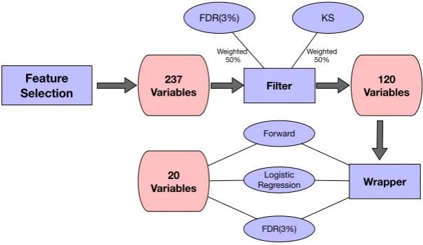
We begin our feature selection process with the universe of 237 expert va-riables created, and first apply our filter methods to reduce the number of expert variables from 237 to 120. By combining the KS and FDR with equal weight, the filter reduces our variable set to about half of the variables, and then we apply the wrapper to reduce to the final 20 variables, still rank-ordered by importance.

Figure 5 illustrates the stages of this two-step feature selection process.

Table 3 below lists the final 20 variables after feature selection.

6. Model Algorithms

(10)

[image:10.595.219.527.74.252.2]

DOI: 10.4236/jilsa.2019.113003 42 Journal of Intelligent Learning Systems and Applications Figure 5. Feature selection process.

Table 3. The selected top 20 variables ranked by importance after feature selection.

Ranking Variables

1 total amount by this cardnum at this merchnum in 7 days 2 max amount by this cardnum in 30 days

3 total amount by this cardnum in this zip code in 14 days 4 actual-median amount by this cardnum in this zip code in 30 days 5 total amount by this merchnum in 1 day

6 total amount by this merchnum in 14 days 7 max amount by this merchnum in 30 days 8 total amount by this merchnum in 7 days

9 total amount by this cardnum at this merchnum in 14 days 10 #transactions by this cardnum in 1 day

11 total amount by this cardnum at this merchnum in 1 day 12 actual/average amount by this cardnum in 30 days 13 #transactions by this cardnum in this state in 1 day 14 max amount by this cardnum in this state in 14 days 15 median amount by this cardnum in this zip code in 30 days 16 median amount by this cardnum in 30 days

17 total amount by this cardnum in this zip code in 30 days 18 actual-average amount by this cardnum in 30 days 19 actual-average amount by this cardnum in 7 days 20 actual/average amount by this merchnum in 30 days

learning methods. For each method, we describe the general principals of the algorithm and the parameter searches performed.

(11)

our data. We use the first 10 months of our data set to build our best models, randomly dividing the records into training and testing in multiple ways, and then we evaluate the model on this out of time data set. This gives us the most likely model performance that will be experienced when the model is imple-mented. Although we use this out of time evaluation multiple times during model tuning, it still provides a more realistic performance expectation measure than what the in-time testing data provides.

6.1. Logistic Regression

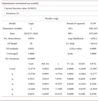
With 20 variables selected, logistic regression functions as a baseline model for its simplicity of parameters interpretation. We note that based on its simplicity and generally fine performance, logistic regression is frequently the method of choice for many real-world business classification problems. For this study, the first step is to build a baseline logistic regression using all variables from our feature selection process. Table 4 below is a summary of the main parameters of this logistic regression model. Each variable xi is the variable given in Table 3.

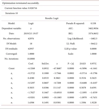
Note that x3 and x16both have p values higher than 0.05, and therefore should

be excluded since they are not statistically significant. Thus the new version of logistic regression on the remaining 18 variables (removing x3 and x16) is shown

[image:11.595.204.535.398.739.2]

in Table 5 summary below.

Table 4. First logistic regression output on the training data.

Optimization terminated successfully. Current function value: 0.026521

Iterations 10

Results: Logit

Model: Logit Pseudo R-squared: 0.539

Dependent variable: y AIC: 3382.435

Date: 2019/2/1 20:01 BIC: 3572.495

No. observations: 62976 Log-Likelihood: −1670.2

Df Model: 20 LL-Null: −3619.4

Df residuals: 62955 LLR p-value: 0.0000

Converged: 1.0000 Scale: 1.0000

No. iterations: 10.0000

Coef. Std. Err. z P > |z| [0.025 0.975] Const −6.3774 0.0952 −66.9633 0.0000 −6.5640 −6.1907

x1 −0.3720 0.0991 −3.7524 0.0002 −0.5664 −0.1777

x2 0.3912 0.0553 7.0703 0.0000 0.2828 0.4997

x3 −0.0651 0.0853 −0.7637 0.4450 −0.2322 0.1020

x4 −0.5262 0.0736 −7.1466 0.0000 −0.6705 −0.3819

(12)

DOI: 10.4236/jilsa.2019.113003 44 Journal of Intelligent Learning Systems and Applications Continued

x6 −1.8396 0.1679 −10.9593 0.0000 −2.1686 −1.5106

x7 −0.8686 0.0907 −9.5745 0.0000 −1.0465 −0.6908

x8 1.6247 0.1464 11.0981 0.0000 1.3378 1.9117

x9 0.8138 0.1118 7.2775 0.0000 0.5947 1.0330

x10 0.9733 0.0953 10.2176 0.0000 0.7866 1.1600

x11 −0.4629 0.0645 −7.1806 0.0000 −0.5892 −0.3365

x12 0.2565 0.0439 5.8379 0.0000 0.1704 0.3426

x13 −0.5733 0.1005 −5.7035 0.0000 −0.7703 −0.3763

x14 0.4198 0.0527 7.9630 0.0000 0.3164 0.5231

x15 −0.1589 0.0636 −2.5002 0.0124 −0.2835 −0.0343

x16 0.0146 0.0536 0.2721 0.7856 −0.0905 0.1197

x17 0.3298 0.0405 8.1483 0.0000 0.2505 0.4091

x18 0.7775 0.0960 8.0953 0.0000 0.5893 0.9658

x19 −0.3247 0.0478 −6.7955 0.0000 −0.4183 −0.2310

[image:12.595.205.538.373.738.2]

x20 0.2963 0.0300 9.8665 0.0000 0.2374 0.3551

Table 5. Final logistic regression output on the training data.

Optimization terminated successfully. Current function value: 0.026716

Iterations 10

Results: Logit

Model: Logit Pseudo R-squared: 0.538

Dependent variable: y AIC: 3402.9056

Date: 2019/2/1 19:57 BIC: 3574.8652 No. observations: 62976 Log-Likelihood: −1682.5

Df Model: 18 LL-Null: −3642.2

Df residuals: 62957 LLR p-value: 0.0000

Converged: 1.0000 Scale: 1.0000

No. iterations: 10.0000

Coef. Std.Err. z P > |z| [0.025 0.975] Const −6.3268 0.0932 −67.8687 0.0000 −6.5096 −6.1441

x1 −0.3722 0.1000 −3.7566 0.0002 −0.5714 −0.1796

x2 0.4580 0.0533 8.5863 0.0000 0.3534 0.5625

x3 −0.5297 0.0607 −8.7208 0.0000 −0.6488 −0.4107

x4 0.5835 0.0386 15.1147 0.0000 0.5078 0.6591

x5 −1.7827 0.1667 −10.6910 0.0000 −2.1095 −1.4559

x6 −0.9201 0.0903 −10.1885 0.0000 −1.0970 −0.7431

(13)

x8 0.7779 0.0893 8.7147 0.0000 0.6030 0.9529

x9 0.9498 0.0906 10.4809 0.0000 0.7722 1.1274

x10 −0.4543 0.0652 −6.9706 0.0000 −0.5820 −0.3265

x11 0.2262 0.0439 5.1566 0.0000 0.1402 0.3122

x12 −0.5552 0.0966 −5.7447 0.0000 −0.7446 −0.3658

x13 0.3950 0.0516 7.6543 0.0000 0.2939 0.4962

x14 −0.1463 0.0581 −2.5207 0.0117 −0.2601 −0.0326

x15 0.2931 0.0405 7.2453 0.0000 0.2138 0.3724

x16 0.7826 0.0943 8.2965 0.0000 0.5977 0.9674

x17 −0.3139 0.0494 −6.3490 0.0000 −0.4108 −0.2170

x18 0.2648 0.0307 8.6278 0.0000 0.2047 0.3250

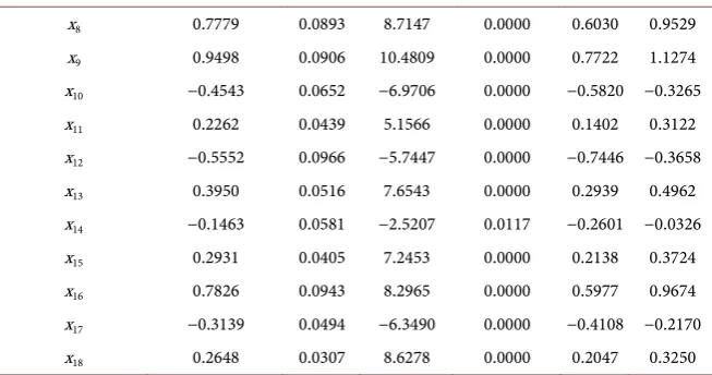
[image:13.595.210.537.84.256.2]

To optimize the logistic regression the number of variables chosen is an ad-justable factor in the tuning process. Models with different numbers of variables are compared in Table 6 below. Note that each experiment of a different num-ber of variables is achieved by removing the last several variables since they are ranked by importance.

Table 6 shows the results of FDR (at 3%) on the out of time data for logistic regression using different numbers of variables, always selected in the rank order shown in Table 3. The nonmonotonic nature of the results is simply a statistical variation due to the sparsity of records.

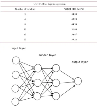
6.2. Artificial Neural Network

An artificial neural network (ANN) is an algorithm that shares simulative struc-ture of the neural network of human brain. As shown in Figure 6. There are an input layer, hidden layers and an output layer in the overall network architec-ture. Each of these layers contains nodes or neurons, which are gathering loca-tions for the receipt and transmission of numerical signals from the previous to the next layer of the neural net. Each neuron embedded in the structure receives a signal from the nodes in the previous layer, applies a transfer function to the signal, and then outputs a new signal to the nodes in the next layer. The signal received from the previous layer is in general a linear combination of the outputs of the previous layer nodes. This combined linear combination signal, received by the node, is then passed through a transfer function, typically a sigmoid or logit function. Other transfer functions are also used, but the sigmoid/logit is the most common.

In this work, we use this sigmoid/logistic nonlinear transfer function, with the equation below.

( )

1

1 e x

S x = ₋ +

( )

(

)

2

( )

(

( )

)

e ₁

1 e

x

S x − S x S x

−

′ = = −

(14)

[image:14.595.208.533.85.445.2]

DOI: 10.4236/jilsa.2019.113003 46 Journal of Intelligent Learning Systems and Applications Table 6. Logistic regression performance for different number of variables.

OOT FDR for logistic regression

Number of variables %OOT FDR (at 3%)

5 44.30

6 45.25

8 44.53

10 31.84

15 34.47

20 39.22

Figure 6. Neural net architecture1_.

The variable x in this equation is the linear combination of the weighted sig-nals received from the nodes in the previous layer.

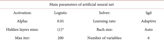
During the parameter tuning process, the key parameters that mainly define the structure of the ANN are number of variables/inputs, hidden layer sizes (number of layers & number of nodes in each layer), a regularization weight al-pha and the learning rate, all of which become the searchable parameters in our tuning experiments. Table 7 below shows the parameters settings of the optimal ANN after tuning.

We note that, even though this was our best ANN model it is likely not the best possible. With only one node in a single hidden layer and the logit trans-form function, it is mathematically equivalent to a logistic regression.

6.3. Support Vector Machine

A Support Vector Machine (SVM) is a wildly applied binary classifier for super-vised machine learning problems. The main characteristics of the SVM algo-rithm are:

(15)

[image:15.595.211.539.89.174.2]

DOI: 10.4236/jilsa.2019.113003 47 Journal of Intelligent Learning Systems and Applications Table 7. Final parameters for the Artificial Neural Net model.

Main parameters of artificial neural net

Activation: Logistic Solver: Sgd

Alpha: 0.01 Learning rate: Adaptive Hidden layers sizes: (1)* Bach size: Auto

Max iter: 200 Number of variables: 6

*layer: 1 nodes: 1.

• _{Expand the dimensionality;}

• _{Look for a linear classifier separation surface in this higher dimensional space.}

It is counterintuitive to expand the dimensionality of a nonlinear machine learning algorithm, since as we argued previously, dimensionality is in a sense the enemy of nonlinear modeling. Expanding the dimensionality can provide new variables, such as the many varieties of the products and higher order pow-ers of the original variables, where a linear separation in this complex higher dimensional space might be a good separation surface. But adding these dimen-sions is against the principals recognized by the curse of dimensionality.

The SVM algorithm achieves this balance by not using explicit new variables in this extended dimensionality, but introduces “virtual” new variables through the use of a kernel trick. It is observed that as the algorithm searches for the best linear separator in the space, all that is needed is some measure of distance. The kernel is a generalized measure of distance and can be employed in this virtual higher dimension without explicitly calculating new variables or explicitly ex-panding the space.

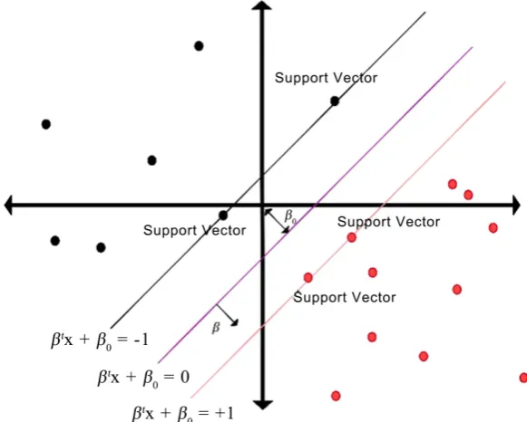
Another important characteristic of the SVM algorithm is the use of a margin concept, where the best linear classifier is selected not just on the basis of the classification error but also considering the best spread around the data, tilting the surface so that this margin of classification/misclassification is as optimal as possible. This is shown in Figure 7.

The choice of a radial basis function (RBF) kernel function is used in this study. The number of variables, C and gamma, are key parameters of the SVM algorithm with the RBF kernel. C is a weight for each of the classes, set to one here, and gamma is a scale factor for the width of the radial basis functions. Ta-ble 8 below shows the final settings of parameters of the SVM after tuning.

6.4. Random Forest

(16)

[image:16.595.225.516.74.307.2]

DOI: 10.4236/jilsa.2019.113003 48 Journal of Intelligent Learning Systems and Applications Figure 7. Support vector machine separation surface2_.

Table 8. Parameter settings for the SVM model.

Main parameters of support vector machine

Kernel: rbf Number of variables: 6

C: 1 Gamma: 1

attempts to separate into two child boxes of the greatest type purity, meaning, the two classes are separated as well as possible. The splitting algorithm contin-ues, considering each child box as a new parent box, and continues to split until a stopping criterion is reached.

Decision trees are an early and ubiquitous machine learning, nonlinear statis-tical modeling methodology. Used extensively decades ago they are known to have serious flaws that are easy to succumb to. The primary deficiency is the tendency to overfit, followed by instability and fragility. The structure of a tree can change substantially depending on near-random choices of the first few splitting locations, which can easily change with small changes in the fitting data set. These deficiencies have been largely overcome through more modern algo-rithms that take advantage of the good properties of trees and greatly avoid these known pitfalls. The use of multiple trees rather than a single complex tree sub-stantially removes many of the problems. Two widely-used architectures that use multiple trees are random forests and boosted trees.

A random forest, shown in Figure 8, is a large collection of decision trees, where the final output is a committee choice across many individual trees. The principle of random forest is that many trees are built, and each uses a random-ly-chosen subset of features. All the results are then combined, typically by

[image:16.595.208.538.361.410.2]

(17)

[image:17.595.235.515.68.317.2]

DOI: 10.4236/jilsa.2019.113003 49 Journal of Intelligent Learning Systems and Applications Figure 8. Random forest architecture.

averaging or voting. A random forest, as compared to a single decision tree, can get a more accurate prediction. Further, since the tree depths are usually smaller and many trees are combined, overfitting issues are largely avoided. While tun-ing the parameters it is important to know what each parameter means. There are 5 important parameters that can be tuned for the random forest algorithm selected:

• _{max_features: Maximum number of features the random forest can try in}

each individual tree;

• _{max_depth: Maximum depth of each tree;}

• _{min_samples_leaf: The minimum number of samples required to split an}

in-ternal node;

• _{n_estimator: Number of trees to be built.}

After multiple trials, the setting of parameters was finalized as is shown in

Table 9 below.

6.5. Boosted Tree

Boosted trees or gradient boosting trees is a type of supervised model that again uses a collection of decision trees, but constructed in a very different way from the random forest. As shown in Figure 9, the boosting process is an iterative approximation process, where we incrementally add more trees, in a fashion similar fashion to a Taylor series, each adding slightly more predictive power to the whole.

(18)

[image:18.595.208.540.87.283.2]

DOI: 10.4236/jilsa.2019.113003 50 Journal of Intelligent Learning Systems and Applications Table 9. Parameter settings for the random forest model.

Final parameter choices of the random forest

Max depth: 5 Max features: 6

[image:18.595.206.541.89.281.2]

Min sample leaf: 2 Min sample split: 10 Estimator: 400 Number of variables: 8

Figure 9. Boosted tree architecture.

for each record, and this error becomes a weighting factor for the next training iteration. Thus as this series of weak learners continues, each next additive tree tends to focus its learning objective on the records for which there is the largest error so far. The use of the latest error as the weights for the next training itera-tion is what gives the algorithm the name boosting, and indeed any weak learner can be used in a boosting algorithm.

Boosted tree models have a set of parameters that can be tuned to improve the quality of the series of weak learners. Some important parameters were explored, specifically the parameters.

Max_depth: Maximum depth of a tree. Increasing this value will make the model more complex and more likely to overfit.

Learning_rate: Step size shrinkage used for the next iterative tree and can help to prevent overfitting. Empirically it has been found that using small learning rates yields dramatic improvements in the model’s generalization ability over gradient boosting without shrinking.

Scale_pos_weight: Control the balance of positive and negative class weights, useful for unbalanced classes.

Min_child_weight: Minimum sum of instance weight (hessian) needed in a child. If the tree partition step results in a leaf node with the sum of instance weights less than min_child_weight, then the building process will give up fur-ther partitioning.

Table 10 below illustrates the final settings of these parameters for the boosted tree after tuning.

7. Model Results

Table 11 below summarizes the FDR at 3% for each model.

(19)

[image:19.595.208.540.89.140.2]

DOI: 10.4236/jilsa.2019.113003 51 Journal of Intelligent Learning Systems and Applications Table 10. Parameter settings for the boosted tree model.

Main parameters of boosted tree

Learning rate: 0.01 Number of trees: 300 Max depth: 5 Number of variables: 20

Table 11. Model results on the card transaction data on the training, testing and out of time validation data sets. These numbers are averages over 10 runs for each data set.

Model FDR (at 3%)

Train (%) Test (%) OOT (%) Logistic regression 72.85 72.96 45.25 Artificial neural net 72.65 68.95 44.86 Support vector machine 90.12 82.29 47.54 Random forest 80.97 79.58 45.42 Boosted tree 89.86 90.08 49.83

can handle the real-time data flow required for a credit card transaction fraud model. The out of time (OOT) data set is set aside, separated from the train-ing/testing data, to simulate how the model will perform when implemented. Thus, the key measure to determine which nonlinear model to deploy is natu-rally the FDR performance on OOT data. Obviously, the boosted tree (FDR = 49.83%) slightly outperformed the next best model (SVM, FDR = 47.54%) and become our best choice for our nonlinear model.

Having settled on the boosted tree as our final model we then examined the FDR at different population cutoff locations, separately on training set, testing set and OOT data set. Tables 12-14 below illustrate these results. Here the FPR is the false positive ratio, the number of incorrectly flagged non-frauds divided by the correctly caught frauds, another common measure of model goodness.

[image:19.595.212.539.186.304.2]

(20)

[image:20.595.57.537.94.519.2]

DOI: 10.4236/jilsa.2019.113003 52 Journal of Intelligent Learning Systems and Applications Table 12. Training results.

Training

#Records #Goods #Bads Fraud rate

62,976 62,339 637 0.0101

Bin statistics Cumulative statistics

Population

bin% #Records #Goods #Bads %Goods %Bads

Total #records

records

Cumulative

good Cumulative bad %Good (FDR) %Bad KS FPR

1 630 90 540 14.3 85.7 630 90 540 0.14 84.77 84.63 0.1667 2 630 601 29 95.4 4.6 1260 691 569 1.11 89.32 88.22 1.2144 3 630 628 2 99.7 0.3 1890 1319 571 2.12 89.64 87.52 2.3100 4 630 627 3 99.5 0.5 2520 1946 574 3.12 90.11 86.99 3.3902 5 630 629 1 99.8 0.2 3150 2575 575 4.13 90.27 86.14 4.4783 6 630 630 0 100.0 0.0 3780 3205 575 5.14 90.27 85.13 5.5739 7 630 628 2 99.7 0.3 4410 3833 577 6.15 90.58 84.43 6.6430 8 630 627 3 99.5 0.5 5040 4460 580 7.15 91.05 83.90 7.6897 9 630 630 0 100.0 0.0 5670 5090 580 8.17 91.05 82.89 8.7759 10 630 618 12 98.1 1.9 6300 5708 592 9.16 92.94 83.78 9.6419 11 630 624 6 99.0 1.0 6930 6332 598 10.16 93.88 83.72 10.5886 12 630 625 5 99.2 0.8 7560 6957 603 11.16 94.66 83.50 11.5373 13 630 630 0 100.0 0.0 8190 7587 603 12.17 94.66 82.49 12.5821 14 630 630 0 100.0 0.0 8820 8217 603 13.18 94.66 81.48 13.6269 15 630 630 0 100.0 0.0 9450 8847 603 14.19 94.66 80.47 14.6716 16 630 627 3 99.5 0.5 10,080 9474 606 15.20 95.13 79.94 15.6337 17 630 630 0 100.0 0.0 10,710 10,104 606 16.21 95.13 78.93 16.6733 18 630 630 0 100.0 0.0 11,340 10,734 606 17.22 95.13 77.91 17.7129 19 630 630 0 100.0 0.0 11,970 11,364 606 18.23 95.13 76.90 18.7525 20 630 629 1 99.8 0.2 12,600 11,993 607 19.24 95.29 76.05 19.7578

Table 13. Testing results.

Testing

20,993 20,750 243 0.0116

Bin statistics Cumulative statistics

Population

bin% #Records #Goods #Bads %Goods %Bads

Total #records

records

Cumulative

good Cumulative bad %Good %Bad (FDR) KS FPR

[image:20.595.57.536.551.730.2]

(21)

[image:21.595.57.538.352.725.2]

6 210 210 0 100.0 0.0 1260 1040 220 5.01 90.53 85.52 4.7273 7 210 208 2 99.0 1.0 1470 1248 222 6.01 91.36 85.34 5.6216 8 210 209 1 99.5 0.5 1680 1457 223 7.02 91.77 84.75 6.5336 9 210 210 0 100.0 0.0 1890 1667 223 8.03 91.77 83.74 7.4753 10 210 209 1 99.5 0.5 2100 1876 224 9.04 92.18 83.14 8.3750 11 210 206 4 98.1 1.9 2310 2082 228 10.03 93.83 83.79 9.1316 12 210 210 0 100.0 0.0 2520 2292 228 11.05 93.83 82.78 10.0526 13 210 210 0 100.0 0.0 2730 2502 228 12.06 93.83 81.77 10.9737 14 210 210 0 100.0 0.0 2940 2712 228 13.07 93.83 80.76 11.8947 15 210 209 1 99.5 0.5 3150 2921 229 14.08 94.24 80.16 12.7555 16 210 209 1 99.5 0.5 3360 3130 230 15.08 94.65 79.57 13.6087 17 210 209 1 99.5 0.5 3570 3339 231 16.09 95.06 78.97 14.4545 18 210 210 0 100.0 0.0 3780 3549 231 17.10 95.06 77.96 15.3636 19 210 209 1 99.5 0.5 3990 3758 232 18.11 95.47 77.36 16.1983 20 210 210 0 100.0 0.0 4200 3968 232 19.12 95.47 76.35 17.1034

Table 14. OOT results.

Out of time

12,427 12,248 179 0.0144

Bin statistics Cumulative statistics Population

(22)

8. Conclusions and Further Work

In this paper, we explore the application of linear and nonlinear statistical and machine learning models on credit card transaction data. The models we build are supervised fraud models that attempt to identify which transactions are most likely fraudulent.

As we would expect, the nonlinear models slightly outperform the linear model, except for the artificial neural network. We believe this underperfor-mance is due to 2 reasons. First, we recognize that we have likely not sufficiently tuned the neural net model and improvement can be found with a different set of model parameters. Second, we note that the data set is substantially limited, and only has 179 labeled fraud events in this OOT data set. The results of any model, particularly a nonlinear one, can be volatile and sensitive to the statistical aberrations and the variation of model parameters. The boosted tree model per-forms the best and can detect about half of the fraud attempts within only the top 3% data that was sorted as suspicious by the fraud algorithm score.

The resulting model can be utilized in a credit card fraud detection system. We note that similar model development process can be performed in related business domains such as insurance and telecommunications, to avoid or detect fraudulent activity.

We also found that we can use the scores of statistical significance in the logis-tic regression models as the criteria for selecting variables: high statislogis-tical signi-ficance score or the low p-value means strong correlation between fraud and re-lated variable. It was found that the logistic regression model works quite well, once sufficiently good expert variables are constructed, which is also seen quite often in practice. What is observed in practice is that well-designed linear models are difficult to beat even with sophisticated nonlinear algorithms. The most impor-tant step is the construction of good expert variables that encode the signals of the problem dynamics as much as possible into clever variables. It is for this reason that linear and logistic regression models are so prevalent in the business field.

More data with more fields (for example, adding point of sale information, time of day, or other cardholder or merchant information) would certainly allow model performance improvements. Further model parameter tuning would also provide improvements to any of the models.

Acknowledgements

The authors would like to thank the Torhea Online Education Research Program as sponsors and hosts for this research project.

Conflicts of Interest

The authors declare no conflicts of interest regarding the publication of this paper.

References

(23)

The Elements of Statistical Learning, Springer, New York, 337-387.

[2] Jensen, D. (1997) Prospective Assessment of AI Technologies for Fraud Detection: A Case Study. In: The AAAI Workshop on AI Approaches to Fraud Detection and Risk Management, AAAI Press, Palo Alto, CA, 34-38.

[3] Randhawa, K., Loo, C.K., Seera, M., Lim, C.P. and Nandi, A.K. (2018) Credit Card Fraud Detection Using AdaBoost and Majority Voting. IEEE Access, 6, 14277-14284. https://doi.org/10.1109/ACCESS.2018.2806420

[4] Ryan, J., Lin, M.-J. and Miikkulainen, R. (1998) Intrusion Detection with Neural Networks. In: Advances in Neural Information Processing Systems, MIT Press, Cambridge, MA, 943-949.

[5] Worldpay (2015) Global Payments Report 2015.

http://offers.worldpayglobal.com/rs/850-JOA-856/images/GlobalPaymentsReportN

ov2015

[6] HSN Consultants (2016) The Nilson Report.

https://www.nilsonreport.com/upload/content_promo/The_Nilson_Report_10-17-2

016.pdf

[7] Stolfo, S., Fan, D.W., Lee, W., Prodromidis, A. and Chan, P. (1997) Credit Card Fraud Detection Using Meta-Learning: Issues and Initial Results. AAAI-97 Work-shop on Fraud Detection and Risk Management, Providence, RI, 27-28 July 1997, 83-90.

[8] Wang, S. (2010) A Comprehensive Survey of Data Mining-Based Accounting-Fraud Detection Research. 2010 International Conference on Intelligent Computation Technology and Automation, Changsha, 11-12 May 2010, 50-53.

https://doi.org/10.1109/ICICTA.2010.831

[9] Sherman, E. (2002) Fighting Web Fraud. Newsweek, 139, 32B.

[10] Green, B.P. and Choi, J.H. (1997) Assessing the Risk of Management Fraud through Neural Network Technology. Auditing, 16, 14-28.

[11] Albashrawi, M. (2016) Detecting Financial Fraud Using Data Mining Techniques: A Decade Review from 2004 to 2015. Journal of Data Science, 14, 553-569.

[12] Dal Pozzolo, A., Caelen, O., Le Borgne, Y.-A., Waterschoot, S. and Bontempi, G. (2014) Learned Lessons in Credit Card Fraud Detection from a Practitioner Pers-pective. Expert Systems with Applications, 41, 4915-4928.

https://doi.org/10.1016/j.eswa.2014.02.026

[13] Estévez, P.A., Held, C.M. and Perez, C.A. (2006) Subscription Fraud Prevention in Telecommunications Using Fuzzy Rules and Neural Networks. Expert Systems with Applications, 31, 337-344. https://doi.org/10.1016/j.eswa.2005.09.028

[14] Fawcett, T. and Provost, F. (1997) Combining Data Mining and Machine Learning for Effective Fraud Detection. Proceedings of AI Approaches to Fraud Detection and Risk Management, 14-19.

[15] Kumari, P. and Mishra, S.P. (2019) Analysis of Credit Card Fraud Detection Using Fusion Classifiers. In: Behera, H., Nayak, J., Naik, B. and Abraham, A., Eds., Com-putational Intelligence in Data Mining. Advances in Intelligent Systems and Com-puting, Springer, Singapore, 111-122.

https://doi.org/10.1007/978-981-10-8055-5_11

[16] Navneet Jain, V.K. (2018) Credit Card Fraud Detection Using Recurrent Attributes.

International Advanced Research Journal in Science, Engineering and Technology, 5, 43-47.

(24)

InformaticaEconomica, 16, 110.

[18] Vardhani, P.R., Priyadarshini, Y.I. and Narasimhulu, Y. (2019) CNN Data Mining Algorithm for Detecting Credit Card Fraud Soft Computing and Medical Bioinfor-matics. Springer, Singapore, 85-93.https://doi.org/10.1007/978-981-13-0059-2_10 [19] Wheeler, R. and Aitken, S. (2000) Multiple Algorithms for Fraud Detection. In:

El-lis, R., Moulton, M. and Coenen, F., Eds., Applications and Innovations in Intelli-gent Systems VII, Springer, London, 219-231.

https://doi.org/10.1007/978-1-4471-0465-0_14

[20] Xuan, S., Liu, G., Li, Z., Zheng, L., Wang, S. and Jiang, C. (2018) Random Forest for Credit Card Fraud Detection. 2018 IEEE 15th International Conference on Net-working, Sensing and Control, Zhuhai, 27-29 March 2018, 1-6.

https://doi.org/10.1109/ICNSC.2018.8361343

[21] Yee, O.S., Sagadevan, S. and Malim, N.H.A.H. (2018) Credit Card Fraud Detection Using Machine Learning as Data Mining Technique. Journal of Telecommunica-tion, Electronic and Computer Engineering, 10, 23-27.

(25)

Appendix: List of 237 Candidate Expert Variables

#transactions with same cardnum in 1 day/average daily #transactions for this cardnum in 7 days #transactions with same cardnum in 1 day/average daily #transactions for this cardnum in 14 days #transactions with same merchnum in 1 day/average daily #transactions for this merchnum in 7 days #transactions with same merchnum in 1 day/average daily #transactions for this merchnum in 14 days #transactions with same merchnum in 1 day/average daily #transactions for this merchnum in 30 days #transactions with same cardnum in 1 day/average daily #transactions for this cardnum in 30 days maximum amount by this cardnum in 30 days

total amount by this cardnum in 30 days median amount by this cardnum in 30 days median amount by this merchnum in 30 days

median amount by this cardnum at this merchnum in 30 days median amount by this cardnum in this zip code in 30 days median amount by this cardnum in this state in 30 days total amount by this merchnum in 30 days

total amount by this cardnum at this merchnum in 30 days total amount by this cardnum in this zip code in 30 days total amount by this cardnum in this state in 30 days maximum amount by this cardnum in this state in 30 days maximum amount by this cardnum in this zip code in 30 days maximum amount by this cardnum at this merchnum in 30 days maximum amount by this merchnum in 30 days

average amount by this merchnum in 30 days

average amount by this cardnum at this merchnum in 30 days average amount by this cardnum in this zip code in 30 days average amount by this cardnum in this state in 30 days average amount by this cardnum in 30 days

#transactions with same cardnum in 30 days #transactions with same merchnum in 30 days

#transactions with same cardnum and merchnum in 30 days #transactions with same cardnum and zip code in 30 days #transactions with same cardnum and state in 30 days #transactions with same cardnum in 1 day/30 days #transactions with same merchnum in 1 day/30 days actual-average amount by this cardnum in 30 days

actual by this merchnumedian amount by this cardnum in 30 days actual/average amount by this cardnum in 30 days

(26)

actual/total amount by this cardnum in 30 days actual/median amount by this cardnum in 30 days actual-average amount by this merchnum in 30 days actual amount by this merchnum in 30 days actual/average amount by this merchnum in 30 days actual/maximum amount by this merchnum in 30 days actual/total amount by this merchnum in 30 days actual/median amount by this merchnum in 30 days

actual-average amount by this cardnum at this merchnum in 30 days actual/average amount by this cardnum at this merchnum in 30 days actual-average amount by this cardnum in this zip code in 30 days actual-average amount by this cardnum in this state in 30 days actual amount by this cardnum in this zip code in 30 days actual/average amount by this cardnum in this zip code in 30 days actual/maximum amount by this cardnum in this zip code in 30 days actual/total amount by this cardnum in this zip code in 30 days actual/median amount by this cardnum in this zip code in 30 days actual amount by this cardnum in this state in 30 days

actual/average amount by this cardnum in this state in 30 days actual/maximum amount by this cardnum in this state in 30 days actual/total amount by this cardnum in this state in 30 days actual/median amount by this cardnum in this state in 30 days actual amount by this cardnum at this merchnum in 30 days

actual/maximum amount by this cardnum at this merchnum in 30 days actual/total amount by this cardnum at this merchnum in 30 days actual/median amount by this cardnum at this merchnum in 30 days total amount by this cardnum at this merchnum in 1 day

(27)

(28)

actual-median amount by this cardnum in this zip code in 14 days actual-median amount by this cardnum at this merchnum in 14 days actual-median amount by this cardnum at this merchnum in 7 days actual-median amount by this cardnum at this merchnum in 1 day actual/median amount by this cardnum at this merchnum in 1 day actual/median amount by this cardnum at this merchnum in 7 days actual/median amount by this cardnum at this merchnum in 14 days actual/median amount by this cardnum in this zip code in 14 days actual/median amount by this cardnum in this zip code in 7 days actual/median amount by this cardnum in this zip code in 1 day

Current transaction date - date of most recent transaction with same cardnum and state Current transaction date - date of most recent transaction with same cardnum and zip Current transaction date - date of most recent transaction with same cardnum and merchnum Current transaction date - date of most recent transaction with same cardnum

Current transaction date - date of most recent transaction with same merchnum average amount by this cardnum in this state in 1 day

(29)

actual/maximum amount by this cardnum in this state in 14 days actual/total amount by this cardnum in this state in 1 day actual/total amount by this cardnum in this state in 7 days actual/total amount by this cardnum in this state in 14 days actual/median amount by this cardnum in this state in 1 day actual/median amount by this cardnum in this state in 7 days actual/median amount by this cardnum in this state in 14 days average amount by this cardnum in 1 day

(30)

actual-median amount by this cardnum in 7 days actual-median amount by this cardnum in 14 days actual-median amount by this merchnum in 1 day actual-median amount by this merchnum in 7 days actual-median amount by this merchnum in 14 days actual/average amount by this cardnum in 1 day actual/average amount by this cardnum in 7 days actual/average amount by this cardnum in 14 days actual/average amount by this merchnum in 1 day actual/average amount by this merchnum in 7 days actual/average amount by this merchnum in 14 days actual/maximum amount by this cardnum in 1 day actual/maximum amount by this cardnum in 7 days actual/maximum amount by this cardnum in 14 days actual/maximum amount by this merchnum in 1 day actual/maximum amount by this merchnum in 7 days actual/maximum amount by this merchnum in 14 days actual/total amount by this cardnum in 1 day actual/total amount by this cardnum in 7 days actual/total amount by this cardnum in 14 days actual/total amount by this merchnum in 1 day actual/total amount by this merchnum in 7 days actual/total amount by this merchnum in 14 days actual/median amount by this cardnum in 1 day actual/median amount by this cardnum in 7 days actual/median amount by this cardnum in 14 days actual/median amount by this merchnum in 1 day actual/median amount by this merchnum in 7 days actual/median amount by this merchnum in 14 days #transactions with same cardnum in 1 day #transactions with same cardnum in 7 days #transactions with same cardnum in 14 days #transactions with same merchnum in 1 day #transactions with same merchnum in 7 days #transactions with same merchnum in 14 days

(31)