Evaluation and Correction of Ground Based Microwave Radiometer Observations Based on NCEP FNL Data

(1)

http://www.scirp.org/journal/acs ISSN Online: 2160-0422

ISSN Print: 2160-0414

DOI: 10.4236/acs.2019.92016 Apr. 1, 2019 229 Atmospheric and Climate Sciences

Evaluation and Correction of Ground-Based

Microwave Radiometer Observations

Based on NCEP-FNL Data

Qing Li

1,2,3*

_{, Ming Wei}

1,2,3

_{, Zhenhui Wang}

1,2,3

_{, Yanli Chu}

4

_{, Lina Ma}

1,2,3

1_{Collaborative Innovation Center on Forecast and Evaluation of Meteorological Disasters, Nanjing University of Information}

Science & Technology, Nanjing, China

2_{Key Laboratory for Aerosol-Cloud-Precipitation, Nanjing University of Information Science & Technology, Nanjing, China}

3_{School of Atmospheric Physics, Nanjing University of Information Science & Technology, Nanjing, China}

4_{Institute of Urban Meteorological Research, CMA, Beijing, China}

Abstract

Consistency between the brightness temperatures observed with a ground-based microwave radiometer and the brightness temperatures computed by forward modeling is important in many different data applications. Using the Nation-al Centers for EnvironmentNation-al Prediction-FinNation-al OperationNation-al GlobNation-al AnNation-alysis (NCEP-FNL) dataset as a reference, the brightness temperature was obtained through the radiation transfer model for forward calculation. The problem of segmented features in long time of observational data from ground-based mi-crowave radiometers (the so-called “jumping problem”) was identified. By analyzing the deviation and correlation between the observational bright temperature data and the forward calculated data under clear sky conditions, a revised scheme is proposed for the bright temperature observational data. Data obtained with a ground-based microwave radiometer in Beijing from January 1, 2010 to December 31, 2011 around the date of liquid nitrogen ca-libration show that the correlation between the observed brightness tempera-tures and the forward computed brightness temperatempera-tures is better after cor-rection, especially at 28 and 30 GHz. The “jumping” problem in the observa-tional data for the brightness temperature is eliminated after correction and the time continuity of the observational data and its consistency with the forward calculated data based on the NCEP-FNL dataset are improved. The proposed correction scheme can be used both for real-time data quality con-trol and to improve the accuracy of historical datasets obtained with poorly calibrated microwave radiometers or radiometers working in polluted envi-ronments.

How to cite this paper: Li, Q., Wei, M., Wang, Z.H., Chu, Y.L. and Ma, L.N. (2019) Evaluation and Correction of Ground-Based Microwave Radiometer Observations Based on NCEP-FNL Data. Atmospheric and Climate Sciences, 9, 229-242.

https://doi.org/10.4236/acs.2019.92016 Received: February 25, 2019 Accepted: March 29, 2019 Published: April 1, 2019

(2)

DOI: 10.4236/acs.2019.92016 230 Atmospheric and Climate Sciences

Keywords

Atmospheric Remote Sensing, Data Correction, Forward Model, Regression

1. Introduction

Ground-based microwave radiometers are commonly used for atmospheric ob-servations [1] and can be operated continuously with a typical temporal resolu-tion of 1 s. They can be used to monitor the temperature and humidity profiles of the atmospheric boundary layer [2]-[9], and unique liquid water content pro-files [10] [11] [12] [13] and to detect lightning [14]. The number of ground-based microwave radiometers in use in China for both research and quasi-operational observations has increased rapidly in recent years [15]-[20] and long time data have been obtained. However, due to changes in the observation position during the monitoring period (changing the environment of the instrument), the depo-sition of atmospheric pollutants on the radome (resulting in lower radome transmittance) and the half-yearly calibration with liquid nitrogen in accordance with the technical requirements of the system (resulting in a discontinuous cali-bration coefficient), these long time observational data show segmented features referred to as the “jumping problem”.

The output from a microwave radiometer is the brightness temperature, which is defined as the electromagnetic energy received by the radiometer at a certain reference frequency. Either inversion processing or data assimilation must be performed to convert the brightness temperature data into information on the atmospheric temperature, humidity and liquid water content profiles based on the theoretical radiative transfer model [21] [22]. The brightness tem-perature observed by the microwave radiometer is inaccurate as a result of the hardware and calibration techniques used and can be solved from the point of view of the hardware. However, corrections to take account of the hardware used and calibration techniques cannot be applied to historical observational data from microwave radiometers and therefore inversion cannot be applied to the temperature and humidity profile. For these historical data, there is no pos-sibility of improving the quality of the hardware to improve data accuracy. This paper discusses whether a data processing method can be used to correct histor-ical observational data. The brightness temperatures observed using a ground-based microwave radiometer and the brightness temperatures simulated using a radia-tive transfer model must be consistent and reconcilable with each other.

(3)

Forecasts model output as the input to the radiative transfer model. They there-fore suggested a correction scheme to improve the application of the FY-3 data. Goldberg etal.[24] found that measurements from the AMSU instrument on-board the NOAA 15 and NOAA 16 satellites varied with the scan angle based on a comparison between the observed and simulated brightness temperatures. Weng etal.[25] showed that there was a clear asymmetry in the measured ra-diance along the scan measured by the AMSU instrument. This was most ob-vious in the window channels and was probably caused by either the misalign-ment of the polarizer or errors in the antenna pointing angle. Weng etal.[26]

concluded that the antenna properties (e.g. the main beam efficiency and the spillover contributions from the side lobes) must be known before computing the brightness temperatures from the antenna temperatures measured by the Advanced Technology Microwave Sounder onboard the Suomi National Po-lar-orbiting Partnership satellite.

Systematic deviations between the observed brightness temperature (TBM) and

the corresponding forward computed brightness temperature (TBC) also exist in

ground-based microwave remote sensing [21], where the difference between the antenna temperature and the brightness temperature in the direction of the beam center is about 2 K for a 6˚ beam width [27]. Meunier etal. [28] studied the effects of the characteristics of the radiometer (e.g. the antenna beam width and the receiver bandwidth) on simulated radiometer measurements based on theoretical simulations in which the beam width calculation is performed using a Gaussian quadrature and neglecting the effects of the side lobes. Tipping calibra-tion is considered to be an important technique for the absolute calibracalibra-tion of ground-based microwave radiometers [27] [29] [30], but this is time consuming and is often not performed as often as would be useful. Wang Z. etal.[31] pro-posed verifying the working status of ground-based microwave radiometers in Nanjing and Wuhan by comparing TBM and TBCon a clear day. Li Qing etal.[32]

tried to correct the systematic deviation to improve the consistency between the

TBM values observed with a 22-channel radiometer in Beijing and the calculated

TBC series for January 1, 2010 to December 31, 2011 when the radiometer was

suspected to be malfunctioning. A liquid nitrogen calibration was performed on December 22, 2010. The results clearly show that the consistency between TBM

and TBC can be improved for most of the 22 channels, but for some channels,

es-pecially channels 7 (28 GHz) and 8 (30 GHz), the improvement in consistency between TBM and TBC is negligible. Further study of this issue is required.

We used the analysis method for the quality control of bright temperature da-ta from a satellite-borne microwave radiometer as a reference. We used NCEP-FNL

[33] dataset as a reference because it has a high accuracy and good representa-tiveness and time-space continuity. These data were used to obtain the bright-ness temperature TBC through the radiation transfer model for forward

calcula-tion [21] [34] [35]. We then identified the “jumping” problem in TBM by

analyz-ing the deviation and correlation between the TBM data and the forward

(4)

TBM. The verification was performed using the observational TBM dataset for the

period January 1, 2010 to December 31, 2011.

2. Theoretical Analysis and Estimation

According to Westwater et al. [21], when the atmosphere is approximated as parallel planar and the scattering can be ignored, the brightness temperature for the thermal radiance vertically downward to the ground is expressed by the ra-diative transfer equation

( )

0

( ) (

0,

)

₀

( ) ( ) ( )

0, d

B B a

T =T ∞ τ ∞ +

∫

∞k z T z τ z z (1)

where

( )

0,z exp

{

₀zka

( )

z dz

}

τ

= −

_∫

′ ′ (2) is the transmittance of the atmosphere from height z to the antenna (z = 0),

( )

0,

τ

∞

_{is the transmittance of the whole atmosphere,}

T

_B

( )

∞

is the cosmic

brightness temperature, which was assumed here to be 2.9 K [21], T z

( )

is the

temperature profile and

k

a

( )

z

is the absorption coefficient due to the presence

of oxygen and water vapor in the atmosphere under a clear sky. ka

( )

z depends

mainly on the pressure, temperature, humidity and wave frequency [36] [37]. The forward calculations according to Equation (1) are based on the radiative transfer model of Westwater et al. [21], including vertical discretization and humidity transformation; the absorption coefficient for atmospheric oxygen and water vapor follows Liebe et al. [37]. Data from either radiosondes or the NCEP-FNL Operational Model Global Tropospheric Analyses [33] can be used as the input temperature and humidity profiles in the forward model. The simu-lation scheme performed well in an earlier series of studies on the quality control and application of ground-based microwave radiometer data [31] [32] [35] [38] [39].

The power obtained by an antenna looking vertically upwards (the antenna temperature) is expressed as [40]:

( ) ( )

( )

4π 4π

, , d , d

A B

T =

∫

T

θ φ

F

θ φ

Ω

∫

F

θ φ

Ω (3)

where θ and

φ

are the zenith and azimuth angles of the incident radiance toward the antenna, dΩ =sin d dθ θ φ,

F

( )

θ φ

,

is the radiation pattern of the

antenna, T_B

( )

θ φ

, is the brightness temperature incident on the antenna from

the direction

( )

θ φ

,

, of which T_B

(

θ=0 , φ

)

is from zenith and is equal to TB(0) defined by Equation (1).

In most situations for a parabolic antenna, F

( )

θ φ

, is approximated to 1 in

the main beam and to 0 elsewhere, so T_A =T_B

( )

0 and Equation (1) can be used

directly to simulate the observations from the antenna.

(5)

[image:5.595.230.527.63.179.2]

DOI: 10.4236/acs.2019.92016 233 Atmospheric and Climate Sciences Figure 1. Schematic diagrams showing (a) the equivalence of the antenna radiation pat-tern; (b) the incident radiance and (c) the influence of the radome.

can correlated with the ambient temperature. Therefore, in order to predict the contamination of the atmospheric radiance measurement from the surroundings with an easy-to-understand formula, we assume that: the values of both F

( )

θ φ

,

and T_B

( )

θ φ

, in the upper hemisphere are isotropic in the azimuth direction;

( )

B

T

θ

in the upward-looking main beam is identical to T_B(0) and is representative

of atmospheric radiance; and TB

( )

θ

in the lower hemisphere is equivalent to

TS and is representative of the radiance from the surroundings (Figure 1(b)).

Equation (3) then becomes

( )

( ) ( )

( )

π 2 π

0 π 2

π

0

1 2 3

2π (0) sin d

2π sin

0

B B S

A

B B S

T F T F T F

T

F d

T T T

α

θ θ θ θ θ θ

θ θ θ

γ θ γ γ

 

 ₊ ₊ 

 

 

 

=

= + +

∫

(4)

where γ1, γ2 and γ3 are parameters determined by the radiation pattern of the

antenna and TB

( )

θ is defined according to the integral mean value theorem. Because the antenna reflector is covered by a metal cover containing a foam dielectric radome (Figure 1(c)), the second term in Equation (4) can be ap-proximated using the contributions from both TB(0) and TS as the proportion β

and hence Equation (4) becomes

(

1

)

(

3 1

)

A B S

T =T

γ β

+ +T

γ

+ −

β

(5)

where T_B =T_B

( )

0 and β is the proportional parameter and depends on the

performance of both the antenna and the radome. A properly maintained or new radome can be taken as a perfect microwave window, but deposits on the radi-ometer radome, especially in areas with high levels of pollution, will increase the opacity of the radome and the value of β will decrease.

According to Equation (5), the observations of atmospheric radiance are in-fluenced by the surroundings and must be corrected. Because the contribution from TS can be mistaken as an increment in TB, the correction to TB to take

ac-count of the surrounding environment according to Equation (5) is

(

3

1 )

(

1

)

B S

T

(6)

surroundings:

*

S g

T ≈εT (7)

where Tg and ε are the surrounding temperature and emissivity, respectively.

3. Verification of the Correction for the Surroundings

To obtain δTB, the amount of correction required to the value of TBM measured

by the radiometer, it is assumed that the surrounding temperature is dominant and the emissivity is combined with

(

γ

3+ −1

β

)

(

γ

1+

β

)

in Equation (6) to

give

B g

T c T

δ = ∗ (8) where c is a coefficient for the correction to the surroundings.

The correction for a systematic deviation caused by the difference between the atmospheric profiles over the radiometer and the atmospheric profiles used as the input in the forward calculation for TBC based on Equation (1) is expressed as

BO BM

T = ∗a T +b

where a and b are coefficients and TBO is the result obtained from the correction

[32]. The combination of the correction for systematic deviations and the cor-rection for the surroundings leads to a bivariate linear regression model

BO BM g

T = ∗a T + + ∗b c T (9)

Considering that the forward calculated result (TBC), based on a radiative

transfer equation such as Equation (1), is mostly used as a reference in data as-similation and profile inversion, let the residual sum of square Q be expressed as

(

)

2

min

BO BC

Q=

∑

T −T = (10)

i.e.,

(

)

(

)

(

)

2 0

BM g BC BM

BM g BC

BM g BC g

Q

a T b c T T T

a Q

a T b c T T

b Q

a T b c T T T

c

∂ ₌ _∗ _{+ + ∗} ₋ _∗ ₌

∂ ∂

= ∗ + + ∗ − =

∂

∂ ₌ _∗ _{+ + ∗} ₋ _{∗ ∆} ₌

∂

∑

(11)

to obtain the optimum estimation for the coefficients a, b and c in Equation (9) from a sample of data.

The data sample used by Li Q. etal. [32] is used here for verification. The data sample is a radiometer with 35 channels, of which 22 are used for observations of the operational brightness temperature. The central frequencies for channels 1 - 8 are 22 - 30 GHz in the K band and the central frequencies for channels 9 - 22 are 51 - 59 GHz in the V band (Table 1). The radiometer has its own thermo-meter for measuring the surface air temperature, which is taken as Tg in the

(7)

[image:7.595.210.537.114.517.2]

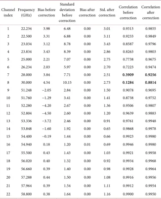
DOI: 10.4236/acs.2019.92016 235 Atmospheric and Climate Sciences Table 1. Bias (K) and standard deviation (std, K) of the difference between the measured and calculated brightness temperatures and their correlation coefficient before and after correction.

Channel

index Frequency (GHz) Bias before correction

Standard deviation before correction

Bias after

correction correction Std. after

Correlation before correction

Correlation after correction

1 22.234 3.98 6.48 0.00 3.01 0.9313 0.9855

2 22.500 3.31 6.88 0.00 3.11 0.9233 0.9849

3 23.034 3.12 8.78 0.00 3.43 0.8587 0.9796

4 23.834 3.43 8.39 0.00 2.86 0.8263 0.9803

5 25.000 2.21 7.07 0.00 2.75 0.7738 0.9675

6 26.234 2.03 5.97 0.00 2.70 0.7223 0.9474

7 28.000 3.84 7.71 0.00 2.51 0.3909 0.9256

8 30.000 4.54 10.15 0.00 2.73 0.1284 0.8814

9 51.248 −2.05 2.84 0.00 1.50 0.9078 0.9695

10 51.760 −1.29 3.41 0.00 1.41 0.8738 0.9752

11 52.280 −4.20 2.67 0.00 1.36 0.9506 0.9807

12 52.804 −4.50 2.60 0.00 1.20 0.9639 0.9883

13 53.336 −3.72 2.46 0.00 0.91 0.9761 0.9948

14 53.848 −1.60 1.92 0.00 0.65 0.9868 0.9978

15 54.400 −0.19 1.44 0.00 0.66 0.9923 0.9980

16 54.940 0.18 1.20 0.01 0.69 0.9946 0.9980

17 55.500 0.43 1.43 0.00 1.03 0.9921 0.9958

18 56.020 0.40 1.32 0.00 0.92 0.9934 0.9968

19 56.660 0.39 1.40 0.00 0.98 0.9928 0.9964

20 57.288 0.44 1.50 0.00 1.08 0.9916 0.9956

21 57.964 0.39 1.54 0.00 1.11 0.9912 0.9954

22 58.800 0.38 1.64 0.00 1.16 0.9900 0.9950

<85% in the troposphere [34]. Only the data for clear sky days were used in the following statistical analysis to avoid the uncertain influence of clouds on the es-timation of the coefficients. However, the results are applicable to all weather conditions because the coefficients account for both the systematic deviations and contamination from the surroundings. Additional corrections may be ne-cessary for the effects of clouds.

1) Verification with time series and correlation analysis

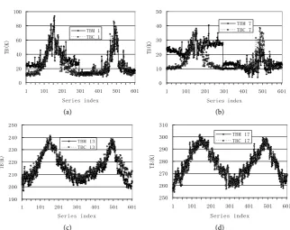
Figure 2 shows the time series of TBM in the sample and the corresponding

simulated values of TBC for four typical channels at 22.234, 28.000, 53.336 and

55.500 GHz. The gap between TBM and TBC includes the error in the radiative

(8)

DOI: 10.4236/acs.2019.92016 236 Atmospheric and Climate Sciences (a) (b)

[image:8.595.212.535.61.316.2]

(c) (d)

Figure 2. Comparison of the time series of the observed clear sky brightness temperatures (TBM) with the simulated temperatures (TBC) for four typical channels during the period

January 1, 2010 to December 31, 2011. (a) Channel 1 (22.234 GHz); (b) Channel 7 (28.000 GHz); (c) Channel 13 (53.336 GHz); (d) Channel 17 (55.500 GHz).

position on the abscissa series index in Figure 2 and another at the 520th posi-tion in the abscissa series index in Figure 2 as a result of the transfer of the in-strument from Shunyi (40˚07'N, 116˚36'E, 34.0 m a.s.l.) to Shangdianzi (40˚39'N, 117˚07'E, 293.3 m a.s.l.). The value of TBM after liquid nitrogen calibration differs

considerably from that before calibration for channels 1 and 7, whereas the value of TBM for channel 13 showed a clear decrease after the instrument had been

moved. The whole sample was therefore sliced into three sub-samples for the correction of TBM.

Based on Equation (11), the coefficients a, b and c were derived from each of the three sub-samples for each of the 22 channels (data not shown) and Equation (9) was applied for correction. Table 1 gives the statistics for the difference be-tween the measured and calculated brightness temperatures and the correlation coefficients before and after correction. The bias before correction was decreased to 0 after correction and the standard deviations all decreased significantly, es-pecially for the channels in the K band. The correlation coefficients between the calculated and measured brightness temperatures after correction were greater than those before correction for all 22 channels, particularly for channels 7 and 8 (as indicated by the bold font in Table 1). The correlation between TBM and TBC

was almost negligible, whereas the correlation between TBO and TBC increased to

about 0.9, mainly due to the correction for the surrounding environment. The improvement in consistency is also shown by the time series for TBO and TBC

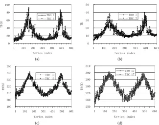
shown in Figure 3 for the same four typical channels, illustrating that this me-thod can be used to improve historical datasets.

0 20 40 60 80 100

1 101 201 301 401 501 601 Series index

TB(K)

TBM 1 TBC 1

0 10 20 30 40 50

1 101 201 301 401 501 601 Series index

TB(K)

TBM 7 TBC 7

190 200 210 220 230 240 250

1 101 201 301 401 501 601 Series index

TB(K)

TBM 13 TBC 13

250 260 270 280 290 300 310

1 101 201 301 401 501 601 Series index

TB(K)

(9)

(a) (b)

[image:9.595.211.537.64.320.2]

(c) (d)

Figure 3. Comparison of the time series of the corrected observed clear sky brightness temperatures (TBO) with the simulated temperatures (TBC) for four typical channels

dur-ing the period January 1, 2010 to December 31, 2011. (a) Channel 1; (b) Channel 7; (c) Channel 13; (d) Channel 17.

2) Verification with temperature and humidity profile retrievals

To verify the corrections to the brightness temperature data, we used the least-squares method to retrieve atmospheric temperature and moisture profiles from TBO and TBM, respectively, and then compared the statistics of the errors in

the retrieved data.

If vector f is the temperature and the water vapor density profiles at L

height levels

[

]

T

1, 2, , L

T T T

=

f  (12)

and vector g is the brightness temperatures at K microwave frequencies

[

]

T

1, 2, ,

B B BK

T T T

=

g  (13)

then the regression equation is

C

= ∗

f g (14)

where C is the regression coefficient matrix, and can be obtained through re-gression analysis by using an a rere-gression sample (of sample size N) of both f

and g based on the least-squares method to give

(

)

2

2 1 1 min N N i i i

Q e C

= =

=

∑

=

∑

f − ∗g =

where f is the temperature and water vapor density provided by the NCEP-FNL

data and g is TBC plus a Gaussian random number according to n(0, σ) to

si-mulate the error in the brightness temperature computations, where σ is the standard deviation given for each channel in Table 1.

0 20 40 60 80 100

1 101 201 301 401 501 601 Series index TB(K) TBO 1 TBC 1 0 10 20 30 40 50

1 101 201 301 401 501 601 Series index TB TBO 7 TBC 7 190 200 210 220 230 240 250

1 101 201 301 401 501 601

Series index TB(K) TBO 13 TBC 13 250 260 270 280 290 300 310

1 101 201 301 401 501 601

Series index

TB(K)

(10)

During the retrieval test with independent samples, TBO and TBM were used to

replace g in Equation (14) and f obtained from Equation (14), respectively.

The first 541 of the 603 samples were used as the regression samples and the last 63 samples were used as the test samples.

The 63 retrievals from TBO and TBM were compared with the NCEP-FNL data

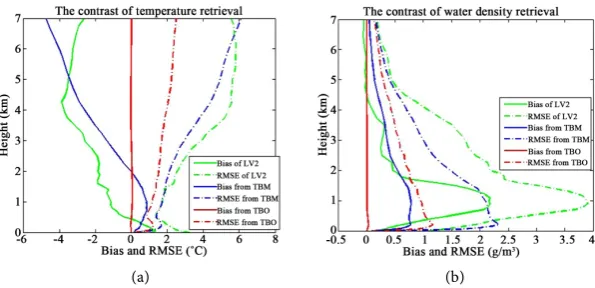
and the error statistics are shown in Figure 4(a) for temperature and in Figure 4(b) for the concentration of water vapor. Figure 4 shows that the bias from TBO

is close to zero and the root-mean-square error (RMSE) is <2˚C for temperature and 1.2 g/m3_{for humidity up to 5 km height. The bias from}_T

BO is better than that

from TBM. This implies that the brightness temperature after correction (TBO) gives

better retrievals than the brightness temperature without correction (TBM).

The radiometer output profiles (LV2) were also compared with the NCEP-FNL data and the bias and RMSE are shown in Figure 4. The bias and RMSE for LV2 are similar to those obtained from and, in some instances, even poorer than those obtained from TBM.

4. Conclusions and Discussion

This work aimed to better preserve the historical data obtained by ground-based microwave radiometers and to improve their value in future applications. We took data from the NCEP-FNL dataset as a reference and then used the radiation transfer model for forward calculation to obtain the brightness temperature. However, we found that long time series of observational data from ground-based microwave radiometers may contain segmented features (the so-called “jumping problem”). Eliminating this “jumping problem” in the brightness temperature observation data will improve both the time continuity of the brightness tem-perature observational data and the consistency of the system with the forward modeled data based on the NCEP-FNL dataset, allowing the observational data to be used for inversion and assimilation at a later date. Our main conclusions are as follows.

[image:10.595.225.523.512.656.2]

(a) (b)

Figure 4. Comparison of error statistics for (a) temperature and (b) concentration of wa-ter vapor. Solid lines show the bias referring to the retrievals from the NCEP-FNL data; dotted lines show the root-mean-square error; green lines show the error statistics for LV2; blue lines show the error statistics for the retrievals from TBM; and red lines show the

(11)

1) The temperature variation around the antenna must be taken into account in the corrections, especially in the K band because the spillover contributions from the side lobes and polluted radome cannot be neglected. Although frequent liquid nitrogen and tipping calibrations of the radiometer system help to alle-viate the interference from the surrounding environment in the brightness tem-perature measurements, it is usually still necessary to correct the observations for this type of interference.

2) Our verification of the two years of observed data shows that our correction scheme is efficient. The consistency between the observations of the atmospheric brightness temperature and the ground-based microwave radiometer and for-ward calculations was greatly improved and the standard deviation of the dif-ference was significantly decreased in all the channels in both the K (20 - 30 GHz) and V (50 - 60 GHz) bands, especially for channels close to 28 - 30 GHz.

3) We verified that the brightness temperature data after correction result in better retrievals of the atmospheric temperature and humidity than the bright-ness temperature data without correction.

Although our comprehensive correction procedure has significantly improved the accuracy of the calculations, this does not mean that the liquid nitrogen and tipping calibrations of the instrument systems are no longer necessary. In areas with high levels of pollution, correct calibration and maintenance of the radi-ometer can mitigate the degradation in the accuracy of the radiradi-ometer and regu-lar cleaning and replacement of the radome are recommended to ensure the op-timum accuracy of the observations. If the correlation and offset between the atmospheric brightness temperature observations and the ground-based micro-wave radiometer and forward calculations are far from the expected values, the radiometer should be suspected of not performing within its specification and should be returned to the factory.

Acknowledgements

The work is jointly supported by the National Natural Science Foundation of China (41675028, 41675029, 41275043, 41005005), The National Basic Research Program (973) of China (2013CB430102), The Project of State Key Laboratory of Severe Weather of Chinese Academy of Meteorological Sciences (2016LASW-B12), and Open Research Funding Program of KLGIS (KLGIS2015A01), Urban Me-teorological Research Foundation IUMKY&UMRF201101 and Program for Postgraduates Research Innovation of Jiangsu Higher Education Institutions (KYLX16_0948). CMA/Institute of Urban Meteorological Research in Beijing provided the observed data twice a day (0800 and 2000BT) during the period from 1 January 2010 to 31 December 2011. Drs. Li Ju, Liu Hongyan, Ruan Shun-xian, Cao Xiaoyan and Mr. Shen Yonghai of this institute help a lot during data processing. NCEP FNL data is obtained from website

(12)

Conflicts of Interest

The authors declare no conflicts of interest regarding the publication of this pa-per.

References

[1] Westwater, E., Crewell, S. and Matzler, C. (2004) A Review of Surface-Based Mi-crowave and Millimeter-Wave Radiometric Remote Sensing of the Troposphere.

RadioScienceBulletin, 77, 59-80.

[2] Cimini, D., Westwater, E.R., Gasiewski, A.J., Klein, M., Leuski, V.Y. and Liljegren, J.C. (2007) Ground-Based Millimeter- and Submillimeter-Wave Observations of Low Vapor and Liquid Water Contents. IEEETransactionsonGeoscienceand Re-moteSensing, 45, 2169-2180.https://doi.org/10.1109/TGRS.2007.897450

[3] Cimini, D., Campos, E., Ware, R., Albers, S., Giuliani, G., Oreamuno, J., Joe, P., Koch, S.E., Cober, S. and Westwater, E. (2011) Thermodynamic Atmospheric Pro-filing during the 2010 Winter Olympics Using Ground-Based Microwave Radiome-try. IEEETransactionsonGeoscienceandRemoteSensing, 49, 4959-4969.

https://doi.org/10.1109/TGRS.2011.2154337

[4] Cimini, D., Nelson, M., Güldner, J. and Ware, R. (2015) Forecast Indices from Ground-Based Microwave Radiometer for Operational Meteorology. Atmospheric MeasurementTechniques, 8, 315-333.https://doi.org/10.5194/amt-8-315-2015 [5] Güldner, J. and Spänkuch, D. (2001) Remote Sensing of the Thermodynamic State

of the Atmospheric Boundary Layer by Ground-Based Microwave Radiometry.

JournalofAtmosphericandOceanicTechnology, 18, 925-933.

https://doi.org/10.1175/1520-0426(2001)018<0925:RSOTTS>2.0.CO;2

[6] Hewison, T. (2007) 1D-VAR Retrievals of Temperature and Humidity Profiles from a Ground-Based Microwave Radiometer. IEEE Transactions on Geoscience and RemoteSensing, 45, 2163-2168.https://doi.org/10.1109/TGRS.2007.898091 [7] Maschwitz, G., Löhnert, U., Crewell, S., Rose, T. and Turner, D.D. (2013)

Investiga-tion of Ground-Based Microwave Radiometer CalibraInvestiga-tion Techniques at 530 hPa.

AtmosphericMeasurementTechniques, 6, 2641-2658.

https://doi.org/10.5194/amt-6-2641-2013

[8] Stähli, O., Murk, A., Kämpfer, N., Mätzler, C. and Eriksson, P. (2013) Microwave Radiometer to Retrieve Temperature Profiles from the Surface to the Stratopause.

AtmosphericMeasurementTechniques, 6, 2477-2494.

https://doi.org/10.5194/amt-6-2477-2013

[9] Illingworth, A., Cimini, D., Gaffard, C., Haeffelin, M., Lehmann, V., Löhnert, U., O’Connor, E. and Ruffieux, D. (2015) Exploiting Existing Ground-Based Remote Sensing Networks to Improve High-Resolution Weather Forecasts.

[10] Ware, R., Solheim, F., Carpenter, R., Güldner, J., Liljegren, J., Nehrkorn, T. and Vandenberghe, F. (2003) A Multi-Channel Radiometric Profiler of Temperature, Humidity and Cloud Liquid. RadiologicScience, 38, 8079-8032.

[11] Ware, R., Cimini, D., Campos, E., Giuliani, G., Albers, S., Nelson, M., Koch, S. E., Joe, P. and Cober, S. (2013) Thermodynamic and Liquid Profiling during the 2010 Winter Olympics. AtmosphericResearch, 132, 278-290.

https://doi.org/10.1016/j.atmosres.2013.05.019

[12] Campos, E.F., Ware, R., Joe, P. and Hudak, D. (2014) Monitoring Water Phase Dy-namics in Winter Clouds. AtmosphericResearch, 147-148, 86-100.

https://doi.org/10.1016/j.atmosres.2014.03.008

(13)

Reehorst, A., Ware, R., McDonough, F. and Politovich, M. (2014) Supercooled Liq-uid Water Content Profiling Case Studies with a New Vibrating Wire Sonde Com-pared to a Ground-Based Microwave Radiometer. Atmospheric Research, 149, 77-87.https://doi.org/10.1016/j.atmosres.2014.05.026

[14] Wang, Z.H., Li, Q., Hu, F.C., Cao, X.F. and Chu, Y.L. (2014) Remote Sensing of Lightning by a Ground-Based Microwave Radiometer. AtmosphericResearch, 150, 143-150.https://doi.org/10.1016/j.atmosres.2014.07.009

[15] Huang, J.P., He, M., Yan, H.R., etal. (2010) A Study of Liquid Water Path and Pre-cipitable Water Vapor in Lanzhou Area Using Ground-Based Microwave Radiome-ter. ChineseJournalofAtmosphericSciences, 34, 548-558.

[16] Liu, H.Y. (2011) The Temperature Profile Comparison between the Ground-Based Microwave Radiometer and the Other Instrument for the Recent Three Years. Acta MeteorologicaSinica, 69, 719-728.

[17] Li, F., Wu, D., Tan, H.B., Bi, X.Y., Jiang, D.H., Deng, T., Chen, H.H. and Deng, X.J. (2012) The Characteristics and Causes Analysis of a Typical Haze Process during the Dry Season over Guangzhou Area: A Case Study. JournalofTropical Meteorol-ogy, 28, 113-122.

[18] Guo, L.J. and Guo, X.L. (2015) Verification Study of the Atmospheric Temperature and Humidity Profiles Retrieved from the Ground-Based Multi-Channels Micro-wave Radiometer for Persistent Foggy Weather Events in Northern China. Acta MeteorologicaSinica, 73, 368-381.

[19] Xu, G., Ware, R., Zhang, W., Feng, G., Liao, K. and Liu, Y. (2014) Effect of Off-Zenith Observation on Reducing the Impact of Precipitation on Ground-Based Microwave Radiometer Measurement Accuracy in Wuhan. AtmosphericResearch, 140-141, 85-94.https://doi.org/10.1016/j.atmosres.2014.01.021

[20] Bao, Y.S., Qian, C., Min, J.Z., Hou, Y.Y. and Lu, Q.F. (2016) 0-10 km Temperature and Humidity Profiles Retrieval from Ground-Based Microwave Radiometer. Jour-nalofTropicalMeteorology, 32, 163-171.

[21] Westwater, E., Wang, Z.H., Grody, N.C. and McMillin, L.M. (1985) Remote Sensing of Temperature Profiles from a Combination of Observations from the Satel-lite-Based Microwave Sounding Unit and the Ground-Based Profiler. Journal of AtmosphericandOceanicTechnology, 2, 97-109.

https://doi.org/10.1175/1520-0426(1985)002<0097:RSOTPF>2.0.CO;2

[22] Solheim, F., Godwin, J., Westwater, E., Han, Y., Keihm, S., Marsh, K. and Ware, R. (1998) Radiometric Profiling of Temperature, Water Vapor, and Cloud Liquid Wa-ter Using Various Inversion Methods. RadioScience, 33, 393-404.

https://doi.org/10.1029/97RS03656

[23] Lu, Q., Bell, W., Bauer, P., Bormann, N., etal. (2010) An Initial Evaluation of FY-3A Satellite Data. ECMWF Technical Memorandum 631, European Centre for Me-dium-Range Weather Forecasts, 58.

[24] Goldberg, M.D., Crosby, D.S. and Zhou, L. (2001) The Limb Adjustment of Amsua Observations: Methodology and Validation. Journal of Applied Meteorologyand Climatology, 40, 70-83.

https://doi.org/10.1175/1520-0450(2001)040<0070:TLAOAA>2.0.CO;2

[25] Weng, F.Z., Zhao, L., Ferraro, R.R., Poe, G., Li, X. and Grody, N.C. (2003) Ad-vanced Microwave Sounding Unit Cloud and Precipitation Algorithms. Radio Science, 38, 8068-8096.https://doi.org/10.1029/2002RS002679

(14)

[27] Han, Y. and Westwater, E.R. (2000) Analysis and Improvement of Tipping Calibra-tion for Ground-Based Microwave Radiometers. IEEETransactionsonGeoscience andRemoteSensing, 38, 1260-1276.https://doi.org/10.1109/36.843018

[28] Meunier, V., Lohnert, U., Kollias, P. and Crewell, S. (2013) Biases Caused by the In-strument Bandwidth and Beam Width on Simulated Brightness Temperature Mea-surements from Scanning Microwave Radiometers. Atmospheric Measurement Techniques, 6, 1171-1187.https://doi.org/10.5194/amt-6-1171-2013

[29] D’orazio, A., DeSario, M., Gramegna, T., et al. (2003) Optimisation of Tipping Curve Calibration of Microwave Radiometer. ElectronicsLetters, 39, 905-906.

https://doi.org/10.1049/el:20030622

[30] Li, J.M., Guo, L.X., Lin, L.K., Zhao, Y.Y. and Cheng, X.H. (2014) A New Method of Tipping Calibration for Ground-Based Microwave Radiometer in Cloudy Atmos-phere. IEEETransactionsonGeoscienceandRemoteSensing, 52, 5506-5513.

https://doi.org/10.1109/TGRS.2013.2290013

[31] Wang, Z.H., Cao, X.F., Huang, J.S., etal. (2014) Analysis on the Working State of a Ground Based Microwave Radiometer Based on Radiative Transfer Model and Me-teorological Data Variation Features. Transactions of Atmospheric Sciences, 37, 1-8.

[32] Li, Q., Hu, F.C., Chu, Y.L., Wang, Z.H., Huang, J.S., Wang, Y. and Zhu, Y.Y. (2014) A Consistency Analysis and Correction of the Brightness Temperature Data Ob-served with a Ground Based Microwave Radiometer in Beijing. RemoteSensing TechnologyandApplication, 29, 547-556.

[33] National Centers for Environmental Prediction/National Weather Service/NOAA/U.S. Department of Commerce (2000) NCEP FNL Operational Model Global Tropos-pheric Analyses, Continuing from July 1999. Research Data Archive at the National Center for Atmospheric Research; Computational and Information Systems Labor-atory, Boulder.

[34] Decker, M.T., Westwater, E.R. and Guiraud, F.O. (1978) Experimental Evaluation of Ground-Based Microwave Radiometric Sensing of Atmospheric Temperature and Water Vapor Profiles. Journal ofApplied MeteorologyandClimatology, 17, 1788-1795.https://doi.org/10.1175/1520-0450(1978)017<1788:EEOGBM>2.0.CO;2 [35] Liebe, H.J., Rosenkranz, P.W. and Hufford, G.A. (1992) Atmospheric 60 GHz

Oxy-gen Spectrum: New Laboratory Measurements and Line Parameters. Journal of QuantitativeSpectroscopy&RadiativeTransfer, 48, 629-643.

https://doi.org/10.1016/0022-4073(92)90127-P

[36] Liebe, H.J. (1985) An Updated Model for Millimeter Wave Propagation in Moist Air. RadioScience, 20, 1069-1089.https://doi.org/10.1029/RS020i005p01069 [37] Ao, X., Wang, Z.H., Xu, G.R., etal. (2013) Study on the Quality Control of

Bright-ness Temperature Data Observed with Ground-Based Microwave Radiometer.

ScientiaMeteorologicaSinica, 33, 130-137.

[38] Wang, Y., Wang, Z.H., Li, Q. and Zhu, Y.Y. (2014) Research of the One-Dimensional Variational Algorithm for Retrieving Temperature and Humidity Profiles from the Ground-Based Microwave Radiometer. ActaMeteorologicaSinica, 72, 570-582. [39] Zhu, Y.Y., Wang, Z.H., Chu, Y.L., Wang, Y. and Li, Q. (2015) Comprehensive

Quality Control on Brightness Temperature Data Observed with a Ground-Based Microwave Radiometer and the Efficiency Analysis. RemoteSensingTechnology& Application, 35, 621-628.