American Journal of Computational Mathematics, 2011, 1, 147-151
doi:10.4236/ajcm.2011.13016 Published Online September 2011 (http://www.SciRP.org/journal/ajcm)
Computing the Moore-Penrose Inverse of a Matrix through
Symmetric Rank-One Updates
Xuzhou Chen1, Jun Ji2
1Department of Computer Science, Fitchburg State University, Fitchburg, USA 2Department of Mathematics and Statistics, Kennesaw State University, Kennesaw, USA
E-mail: xchen@fitchburgstate.edu, jji@kennesaw.edu
Received February 22, 2011; revised April 14, 2011; accepted May 12,2011
Abstract
This paper presents a recursive procedure to compute the Moore-Penrose inverse of a matrix A. The method
is based on the expression for the Moore-Penrose inverse of rank-one modified matrix. The computational complexity of the method is analyzed and a numerical example is included. A variant of the algorithm with lower computational complexity is also proposed. Both algorithms are tested on randomly generated matri-ces. Numerical performance confirms our theoretic results.
Keywords:Finite Recursive Algorithm, Moore-Penrose Inverse, Symmetric Rank-One Update
1. Introduction
The computation of the generalized inverse of a matrix has been discussed by numerous papers, from Newton types of iterative schemes to finite algorithms. In par-ticular, the finite recursive algorithms have been investi-gated by several authors [1-4]. Many of these finite algo-rithms are based on the computation of the generalized inverse of the rank-one modified matrix.
Our aim is to give a new finite recursive algorithm for computing the Moore-Penrose inverse. The approach is based on the symmetric rank-one updates. The work can be viewed as the generalization of an earlier result on the
Moore-Penrose inverse of rank-one modified matrix A +
cd* [5, Theorem 3.1.3]. Numerical tests show that our
approach is very effective to the computation of Moore-Penrose inverses for rectangular matrices.
Throughout this paper we shall use the standard
nota-tions in [5,6]. and stand for the n-dimensional
complex vector space and the set of m matrices over
complex field C respectively. For a matrix
n
C Cm n
n
m n
A C we
denote R(A), N(A), A*, and A† the range, null space,
con-jugate transpose and Moore-Penrose generalized inverse
of A, respectively.
It is well-known that the Moore-Penrose inverse A† of
A can be expressed as A† = (A*A)†A*. Thus, we can write
†
† *
1 m
i i i
where * is the i-th row of A. Define
i r
* 0
1
0, l l i i , 1, 2, , ,
i
A A r r l
m.
(2)
and
† *, 1, 2, ,
l l
X A A l m (3)
Note that Al Al 1 r rl l*
is the rank-one
modifica-tion of Al1. In the next section we will propose a finite
recursive algorithm which effectively computes Xl in
terms of Xl-1 starting from X0 with the help of the existing
rank-one update formulas for the Moore-Penrose inverse.
After m iterations, m† *
m
X A A will be finally reached,
resulting in the Moore-Penrose inverse A† of A due to the
fact that
†
† * * *
1 m
m m i i
i
X A A r r A
* † *A A A
=A†
Our algorithm will never form Al† explicitly and
per-form any matrix multiplications as stated in (3) at each iteration. Thus it has a low computational complexity. The details of its computational complexity will be in-cluded in the paper. To improve its computational com-plexity, a variant is also proposed. A numerical example is presented in Section 4. We also test and compare the efficiencies of Algorithms 1 and 2 by comparing the CPU times on randomly generated matrices of different sizes.
*
A r r A
2. The Finite Recursive Algorithm for
Moore-Penrose Inverse
First, let us establish a relation between
*
†1 l i i
A r r
and †
1 l
A . For each l1, 2, , , m define
† 1 , l l l
k A r
*
l l
h r † 1, l
A
†1 1 ,
l l l
u I A A
rl
(4)
* l l
v r
† 1 1 , l lI A A
*
1
l rl
† 1 . l l
A r
Theorem 1. Let Al( ) and βl be defined as
in (2) and (4) respectively. Then βl≥1 for each l.
1, 2, ,
l m
Proof. Obviously, . We now only
need to prove the result for
* 1 1 r1
2
† 0 1 1 A r
.
l m
Observe that Al =
is positive semi-definite for 1 Let γbe
the rank of l1
* 1 l
i i ir r
l m.A . Then Al1 is unitarily similar to a
diago-nal matrix, i.e.,
* 1
l
A UDU
where U is a unitary matrix and D = diag
1, 2,,with 1 2
0, ,0 0. We can write Al-1† =
UD†U* which is also positive semi-definite due to the
fact that D† = diag
1 2
1 ,1 , ,1
* ,0, † 1 1. l l A r ,0 .
Therefore,
we have βl = 1+rl* □
The general result for the Moore-Penrose inverse of a rank-one modified matrix can be found in [5]. For a
ma-trix , , the Moore-Penrose
inverse of A + cd* can be expressed in terms of A†, c, and
d with six distinguished cases. Our approach is to apply
the result to the sequence (3) where each Al is positive
semi-definite, βl is real and nonzero in view of Theorem
1 which simplifies the theorem by eliminating three cases. Due to the fact that (Al-1†)* = (Al-1*)† = Al-1† we also
have hl = kl* and vl =ul* from which two of three other
cases can be combined into one. Thus, the six cases of [1] are reduced to only two cases. Moreover, the update formulas can be significantly simplified.
m n
A C c C m, d C n
Theorem 2. The Moore-Penrose inverse of Al = Al-1+
rl rl* defined in (2) is as follows.
1) If ul≠0, then
† * * 1 1 † * 1 1 † † 1 1l l l l l l
l l l l l l
l l l l
A r r A r r
A r r A r r
A A u u
(5) and
*
† 1 l l lA r r Al†1k ul l†u k*l† l*l lu u*† †l (6)
2) If ul= 0, then
† * * 1 1 † * * 1 1 † 1 1 † 1 1l l l l l l
l l l l l l
l l
l l
A r r A r r
A r r A r r
A A A A (7) and
*
† 1 l l lA r r † 1 1
l l l
* l
A k k (8)
Proof. The result follows directly from [5, Theorem
3.1.3] and its proof. Details are omitted. □
Finally, let us turn our attention to establishing the
it-erative scheme from Xl−1to Xl. To this end, we define
two auxiliary sequences of vectors ys,t = As†rt and zs,t =
Asys,t= As As†rt. It is easily seen from
* *
*
s s s s s s s s
A A† A A† A A† A A* †
s s A A†
that ys,t and zs,t are the minimum-norm least-squares
solu-tions of the following two auxiliary linear systems re-spectively
, .
s t s s t
A y r A zA r
In what follows we will frequently employ the fact
that a† = a*/||a||2 for any non-zero column vector a. We
will distinguish two cases in our analysis in view of Theorem 2.
Case 1 (ul≠ 0). It is easily seen from Theorem 2 that
*
*1 1
l l l l
l l l l l l l l
X A r r A
X k u A u k A u u A †
† † † † (10)
Note that
1 1 1
*
1 1 1
*
1 1
*
1, 1 1
* 1, 1, 1, * 1, 1, 1,
l l l l l l l
l l l l l
l l l l l
l l l l l l
l l l l
l l l l l
l l l l
l l l l
k u A A r I A A r A
A r r I A A A r r A A r
y r A A r A
r r z
y r z A
r r z
y A r z
† † † † † † † †
* 1, ll l l l r r z
(11)
Similarly, we have
* 1, 1, * * * * 1 l l - l l l l ll l l - ,l
r z Ay
u k A
r r z
X. Z. CHEN ET AL. 149 and
* * * * * -1, 1, *1 * 2
-1, * * 1 -1, 1, 2 * -1, 1 1
l l l
l l l l l l l l l
l l l l l l l
l l l l l l l l l l
u u A
r z r z A
r A r
r r z
r A r
r z A r z r r z
† † † †
(13)Combining (10) through (13), we have
* *
-1, -1, 1, -1,
1 * *
-1, -1, * * 1, -1, 1, 2 * -1, 1
l l l l l l l l l l
l l
l l l l l l l l
l l l
l l l l l l
l l l l
y A r z r z Ay
X X
r r z r r z
r y
r z A r z
r r z
(14) It is seen from Theorem 2 that
* , 1 * * * 1 = .l t l t l l l t
l l l l l l l l
y A r A r r r
t A k u u k u u r † † † † † † †
Thus, we have an iterative scheme for yl,t:
*
1, -1, -1, 1,
, 1, * *
-1, -1, * 1, * -1, 1, 2 * -1, 1
l l l t l t l l l l l t l t l t
l l l l l l l l l l l
l l l l t l t l l l l
y r r z r z r y
y y
r r z r r z
r y
r z r r z r r z
* (15)
For the auxiliary sequence zl,t = Al yl,t, we could
multi-ply Al on both sides of (15) and then simplify the resulted
expression. However, in our derivation we employ (5) instead:
, 1 1 1,
*
1 1 1 1
, *
1 1
l t l l t l l l l t l t l l t l l l l l l t l 1 t
l l l l
z A A r A A u u r z u u r I A A r r I A A r z
r I A A r
† † † † † † †
Therefore, we have
*
1, 1,
, -1, *
1,
.
l l l l t l t l t l t
l l l l
r z r r z
z z
r r z
1,l,
(16)
Case 2. (ul= 0). Observe that
* *
1
1 1
l r A rl l l r yl l
† (17)
* *
1, 1, l l l l l l
k k A y Ay (18) It is seen from Theorem 2 that
*
*
*1 1 1
l l l l l l l l
* *
1 1 ,
l l l l
X k k A
which, together with (17) and (18), implies
*1 * 1,
-1,
1
. 1
l l l l l l
l l l
X X y Ay
r y
-1, (19)
By following the same token, we can develop an itera-tive scheme for yl,t:
* 1,
, 1, * 1
-1,
. 1
l l t
l t l t l l
l l l
r y
y y y
r y , , (20)
For zl,t, in view of (7), we have
, 1 . l t l t
z z (21) Finally, since A0 = 0 we have X0 = 0, y0,t = z0,t = 0 (t =
1,2, ···, m) from which we can compute the
Moore-Pen-rose inverse Xm = A† by applying (14) or (19) repeatedly
with the help of auxiliary sequences yl,t and zl,t (t = l + 1,
l + 2, ···, m and l < m). We summarize this procedure in the following algorithm.
Algorithm 1. MPinverse1[A]
● Step 0 Input: A. Let be the i-th row of A (i = 1,2,
···, m);
* i
r
● Step 1 Initialization: Set X0 = 0 Cn × m, y0,t = z0,t=
0 Cn for all t = 1, 2, ···, m; ● Step 2 For l = 1, 2, ···, m, 1) if rl – zl – 1,l≠0, then
compute Xl using (14);
compute yl,tand zl,t using (15) and (16)
respectively for all t = l + 1, l + 2, ···, m
and l < m;
2) if rl – zl – 1,l = 0, then
compute Xl using (19);
compute yl,tand zl,t using (20) and (21)
respectively for all t = l + 1, l + 2, ···, m
and l < m;
● Step 3 Output: Xm, the Moore-Penrose inverse of A.
Let us analyze the two cases in our algorithm further.
If ul = 0 for some l, which is the case Step 2(b) in our
algorithm, then we have
1 1
* *
1 1 1 1
1 1
.
l l
l l l l i i l l i l l i
i i
r A A r r r A r r A r r
† † †
This means that if ul = 0 for some l, rl is a linear
com-bination of {ri: I = 1, 2, ···, l – 1}. The following
inter-esting result shows that the opposite is also true.
Theorem 3. Let ui and ri(i = 1, 2, ···, m) be defined as
before. Then, ul = 0 if and only if rl is a linear
combina-tion of {r1, r2, ···, rl – 1}.
Proof. The definition of ul = (I – Al–1Al–1†)rl indicates
that ul = 0 is equivalent to rlN(I – Al–1Al–1†). Let Âl–1 =
[r1 |r2| ··· | rl–1]. Obviously, we have Al–1 = Âl–1Âl–1*. It is
easily seen that
* X A r r A A k k A† †
1
1 l
†
.
ˆl1 ˆl1ˆl1
l1
R A R A A R A
R A A
l1 l1
N I A A l .†
Therefore, ul = 0 is equivalent to rlR(Âl–1), i.e., rl is a
linear combination of {r1, r2, ··, rl–1}. □
3. A Variant of the Finite Recursive
Algorithm with an Improved
Computational Complexity
We now compute the computational complexity of Algo-rithm 1, and then discuss a revised algoAlgo-rithm to improve the efficiencies. Let us focus on the multiplications and divisions ignoring the additions and subtractions. We also count the dominant terms only and ignore the lower terms. Assume that the same quantity is computed only once when the algorithm is implemented. For example,
rl*(rl – zl–1,l) in (14) is computed only once and will not
be re-computed in (15)-(16). After optimizing the code,
it is not difficult to see that 4mn operations are need in
(14) and 6n in (15)-(16). In Case 2, 2mn operations are
needed in (19) and 2n in (20)-(21). Therefore, the total
number of operations T is about
0 1 0 1
0 0
4 6 2 2
4 6 2 2
l l
l l
m m
u t l u t l
u u
T mn n mn n
mn n m l mn n m l
Let γ be the rank of A. In view of Theorem 3, there are
exactly γ elements in the set {l: 1≤ l ≤ m, ul≠0} and(m –
γ) elements in its complement set {l: 1≤ l ≤ m, ul=0}.
Therefore, we have
0 2
0 0
2
0 1
2
0
4 6 2 2
2 2 6 2 .
2 2 4 2 1
3 2 4 .
l
l l
l
l u
u u
n
u l
u
T mn n m l mn m n m l
m n mn n m l n m l
m n mn n m l n m
m n mn mn n m l
0 l u
Note that
0
4 4 2
4 1 2
l u
n m l n m l m m
n m
Therefore, after ignoring lower terms, we obtain
2 2
3m n2mn T 3m n6mn22n, (22)
which leads to the following theorem.
Theorem 4. When applied to the matrix A Cm × n,
with roughly T multiplications and divisions where T satisfies (22).
In view of T
Algorithm 1 computes the Moore-Penrose inverse of A
heorem 4, the computational complexity of
then apply Algorithm 1 to A, i.e., X
=
, then apply Algorithm 1 to A. Let Y
=
Penrose inverse A of
A.
Step 2 is called, then the computational complexity of
. Preliminary Numerical Results
e show some numerical results obtained by both
algo-s on a algo-small problem w
Algorithm 1 grows linearly as a function of n.
How-ever, it grows quadratically as a function of m. Thus this
algorithm is very fast for small m and much slower for
large m. Our preliminary numerical tests confirm the
theoretical discovery. Due to the fact that (A*)†= (A†)*,
let us apply Algorithm 1 to A* when m is bigger than n. If
the output of Algorithm 1 on A* is Y, i.e., Y =
MPin-verse1[A*], then we have Y = (A*)† so A† = Y *. We end
up this section with the following algorithm for A†.
Algorithm 2. MPinversel[A]
● Step 0 Input: A;
● Step 1 If m ≤ n,
MPinverse1[A];
● Step 2 If m ≥ n *
MPinverse1[A*] and set X = Y*;
● Step 3 Output: X, the Moore- †
If
Algorithm 2 is bounded by 3mn2+ 6γmn – 2γ2m in
view of Theorem 4 since the roles of m and n are
switched. Therefore, the complexity of Algorithm 2 is
bounded by K where K = 3m2n + 6γmn – 2γ2n if m ≤ n
and K = 3mn2 + 6γmn – 2γ2m if m > n.
4
W
rithms proposed in the previous sections. One major ad-vantage of our algorithms is that they will be guaranteed to carry out a result successfully.
We first illustrate our algorithm ith accurate calculation at each step.
Example 1. Let
1 2 3 4 5 6
A
(23)
By using either one of our algorithms, we generate a sequence of matrices
0 1
2
00 1 14 8 49
00 , 1 7 16 49 ,
00 3 14 24 49
17 18 4 9
1 9 1 9
13 18 2 9
X X
X
(24)
where X2 = A† which is the Moore-Penrose inverse of A.
at
Al-X. Z. CHEN ET AL. 151
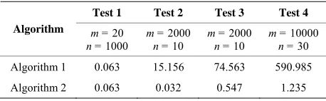
times (in seconds) taken by our al
. Conclusions
[image:5.595.57.286.404.475.2]wo finite recursive algorithms are proposed in this pa-gorithms 1 and 2. The MATLAB Profiler is used in the computation of CPU times for the solution of each prob-lem by each algorithm.
Table 1 records the
or much less columns than rows, the second algorithm is extremely effective according to its computational com-plexity, which is also confirmed by our preliminary nu-merical tests on randomly generated matrices of different sizes.
gorithm on each randomly generated matrix of various sizes. The recorded results coincide with the computa-tional complexity analysis perfectly. Observe that the performances of both algorithms are exactly the same in
Test 1 which is expected due to the fact that Algorithm 2 indeed calls Algorithm 1 in this case. However, in the
case where mn as in Tests 2,3 and, 4, Algorithm 1
is extremely slow as expected from the computational complexity analysis while Algorithm 2 dramatically re-duces the number of operations, thus less time needed for solutions.
The idea in this paper may be adopted to calculate the minimum-norm least-squares solution to the system of
linear equations A x = b.
6. Acknowledgements
The authors are grateful to the referees for their useful comments.
7. References
5
[1] X. Chen, “The Generalized Inverses of PerturbedMatri-ces,” International Journal of Computer Mathematics, Vol. 41, No. 3-4, 1992, pp. 223-236.
T
[2] T. N. E. Greville, “Some Applications of Pseudoinverse of a Matrix,” SIAM Review, Vol. 2, No. 1, 1960, pp. 15-22. doi:10.1137/1002004
per for the Moore-Penrose Inverse of a matrix A Rm×n.
They are based on the expression for the Moore-Penrose inverse of symmetric rank-one modified matrix. The com- putational complexities of both algorithms are analyzed. For matrices with either much less rows than columns
[3] S. R. Vatsya and C. C. Tai, “Inverse of a Perturbed Ma-trix,” International Journal of Computer Mathematics, Vol. 23, No. 2, 1988, pp. 177-184.
doi:10.1080/00207168808803616
Table 1. Computational times (in seconds) for rand
Test 2 Test 3 Test 4
omly
[4] Y. Wei, “Expression for the Drazin Inverse of a 2 × 2 Block Matrix,” Linear and Multilinear Algebra, Vol. 45, 1998, pp. 131-146. doi:10.1080/03081089808818583
generated matrices.
Test 1
[5] S. L. Campbell and C. D. Meyer, “Generalized Inverses of Linear Transformations,” Pitman, London, 1979.
Algorithm m = 20 m m m
n = 1000
= 2000
n = 10
= 2000
n = 10
= 10000
n = 30
[6] G. R. Wang, Y. Wei and S. Qiao, “Generalized Inverses: Theory and Computations,” Science Press, Beijing/New York, 2004.
Algorithm 1 0.063 15.156 74.563 590.985