Lower and Upper Bounds for the Master Bay Planning Problem

Lower and Upper Bounds for the Master Bay Planning Problem

Laura Cruz-Reyes

, Paula Hernández Hernández

, Patricia Melin

, Julio

Mar-Ortiz

, Héctor Joaquín Fraire Huacuja

, Héctor José Puga Soberanes

and Juan Javier

González Barbosa

1

Tecnológico Nacional de México, Instituto Tecnológico de Ciudad Madero,

Tamaulipas, México,

Tecnológico Nacional de México, Instituto Tecnológico de Tijuana,

Baja California, México,

Universidad Autónoma de Tamaulipas. Tampico, Tamaulipas,

México and

Tecnológico Nacional de México, Instituto Tecnológico de León, México

[email protected], [email protected], [email protected],

[email protected], [email protected], [email protected] and

[email protected]

Abstract. In this work we tackle the problem of the stowage of containers on a ship, the so-called Master Bay Planning Problem (MBPP). This is an important hard combinatorial optimization problem in the context of maritime port logistics which has proven to be really difficult to solve. We proposetwo new lower bounds and two new upper bounds which are useful to solve it. In order to test both the efficiency and the effectiveness of the bounds proposed, we conduct an experiment over three different sets of instances. This allows us to determine the specific conditions in which the bounds can be used.

Keywords: Lower bound, upper bound, Master Bay Planning Problem, combinatorial optimization.

1

Introduction

The Master Bay Planning Problem (MBPP) is a combinatorial optimization problem in the context of maritime transportation. Specifically, MBPP consists of finding the best plan to stow a set of containers into another set of available locations of the containership. This problem is really difficult to solve due to the combinatorial nature of alternatives to allocate the containers [1].

When solving integer programs, an important issue is to develop good lower and upper bounds. Their importance lies in the fact that they aid with fathoming and testing for optimality. In integer programming (IP), important solution strategies consist on applying heuristic and relaxation for systematically tightening lower and upper bounds [2].

In this paper we propose two new lower bounds and two new upper bounds for the Master Bay Planning Problem. One of the lower bounds consists of relaxing an integer programming formulation for MBPP. The other three bounds are designed in a heuristic fashion. In order to test both the efficiency and the effectiveness of the lower and upper bounds, we conducted an experiment over three different sets of instances. The results show that some bounds (either lower or upper) are better when only considering either the computational time or the solution quality, independently.

This paper is organized in six sections. Section 2 describes the problem faced. Section 3 describes the new two lower bounds for MBPP. Section 4 presents our proposed upper bounds. Section 5 shows the experimental results and the computational analysis.

Finally, Section 6 shows the conclusions.

2

Problem description

The Master Bay Planning Problem (MBPP) is an NP-hard combinatorial optimization problem [3] which is defined as follows [4]. Let C and S be the set of n containers with different characteristics to be loaded on the ship and the set of m available locations on the containership, respectively. The goal is to assign each container to a location of the ship such that the total stowage time is minimized and all the given structural and operational constraints are satisfied. The 0/1 Linear Programming Model that resumes the problem was proposed by Ambrosino et. al. [5].

In the containership, the l-th location is addressed by the indices i, j, k which represent its bay, row and tier, respectively. We denote by I, J and K, respectively, the set of bays, rows and tiers of the ship, and by b, r and s their corresponding cardinality. The objective value is given by the sum of the times t_lc required for loading each container cC in the corresponding location

S

l , i.e., 



L .

The main constraints that must be considered for the stowage planning process for an individual port are related to the structure of the ship and focused on the size, type, weight, destination and distribution of the containers to be loaded. The description of each constraint is found below.

Size of containers. Usually, set C of containers is the union of two subsets, T and F, consisting, respectively, of 20 and 40 feet containers. Two contiguous locations of 20 feet are required to stow containers of 40 feet. Most of maritime companies number the bays for stowing 40’ containers with even numbers. Such bays actually correspond to two contiguous bays numbered with odd numbers. The odd bays are used for the stowage of containers of 20 feet. Consequently, when a 40’ container is located in an even bay (for instance bay 02), any 20’ container cannot be located in the locations with the same row and tier corresponding to the two contiguous odd bays (e.g. bay 01 and bay 03).

Type of containers. Different types of containers, such as standard, carriageable, reefer, out of gauge and hazardous ones can usually be stowed in a containership. The location of reefer containers is defined by the ship coordinator (who has a global vision of the trip). Hazardous containers are also assigned by the harbormaster’s office, which authorizes their loading. In particular, hazardous containers cannot be stowed either in the upper deck or in adjacent locations.

Weight of containers. The standard weight of an empty container ranges from 2 to 3.5 tons, while the maximum weight of a full container to be stowed in a containership ranges from 20–32 and 30–48 tons for 20’ and 40’ containers, respectively. The weight constraints force the weight of a stack of containers to be less than a given tolerance value. In particular, the weight of a stack of 3 containers of 20’ and 40’ cannot be greater than an a priori established value, say MT and MF,respectively. Moreover, the weight of a container located in a tier cannot be greater than the weight of the container located in a lower tier having the same row and bay and, as it is always required for security reasons, both 20’ and 40’ containers cannot be located over empty locations.

Destination of containers. A good general stowing rule suggests to load first (i.e., in the lower tiers) those containers having as destination the final stop of the ship and load last those containers that have to be unloaded first.

Distribution of containers. These constraints, also known as stability constraints, are related to a proper weight distribution in the ship. In particular, we have to verify different kinds of equilibrium, namely:

 Horizontal equilibrium: the weight on the right side of the ship, must be equal (within a given tolerance, say Q₁) to the weight on the left side of the ship. L and R are the sets of rows belonging to the left and right side of the ship, respectively.

 Cross equilibrium: the weight on the stern must be equal (within a given tolerance, say Q₂) to the weight on the bow. A and P are the sets of anterior (bow) and posterior (stern) bays of the ship, respectively.

3

Lower bounds

A lower bound (LB) is a value indicating that the optimal value of an instance must be greater than it. A lower bound is considered tight when it is close to the optimum. A tight lower bound allows reducing the exploration of the search space by avoiding solutions whose objective value is less than LB.

As far as we know, fast methods to compute lower bounds for MBPP have not been proposed. However, lower bounds for other kind of stowage problems have been reported [6]. In this section we describe two lower bounds for the Master Bay Planning Problem.

3.1. Estimation of the minimal loading time (LB1)

This lower bound consists of allocating all the containers in the locations whose loading times are minimal. The reason for selecting these locations is that the objective function requires minimizing the total loading time. It is important to mention that LB1 only verifies the satisfaction of the constraint concerning to the size of containers. If all constraints were verified by LB1, it would probably select the locations whose loading times are not minimal. Algorithm 1 shows the pseudocode of LB1. Notice that LB1 is computed deterministically.

Algorithm 1. Pseudocode of LB1.

1. Split the set of containers C according to the type of each container. This splitting generates two subsets: T for containers whose size is 20 feet and F for containers whose size is 40 feet. 2. Sort the set of locations S by the loading time associated to each

location in ascending order.

3. First, stow all the containers in T into the first available locations recently sorted. Then, stow all the containers in F into the first remaining locations.

4. Compute the loading time resulting from the stowage plan.

3.2. LP relaxation (LB2)

A linear programming problem (LP)is a class of the mathematical programming problem, which is a constrained optimization problem. In order to solve a linear program, we need to find a set of values for continuous variables (x₁,x₂,...,x_n) that maximizes or minimizes a linear objective functionz. These values must alsosatisfy a set of linear constraints, which consists of a system of simultaneous linear equations and/or inequalities [2].

An integer (linear) programming problem (IP) is a linear programming problem in which at least one of the variables is restricted to integer values [2]. In general, obtaining an optimal solution for an IP formulation is NP-hard [7]. Therefore, tight lower and upper bounds become really important to reduce the computational effort employed to solve such IP models.

An LP-relaxation is obtained by relaxing the integrality constraints of an IP model [7]. This LP-relaxation is important since it can be solved in polynomial time and the solution can be used as a bound on the original IP formulation [8]. In this research we use the LP-relaxation of the IP model for MBPP proposed by Ambrosino et al. in [5] in order to obtain a lower bound to the problem. The basic steps involved to obtain the LP-relaxation are the following:

1) Relax the integer constraints (usually 0–1 constraints on decision variables) to continuous constraints. For example, an integer constraint x_ij{0,1} would be replaced by 0x_ij1.

4

Upper bounds

An upper bound (UB) is a value higher than the optimum of an instance in an optimization problem. An upper bound near the optimum, that is, a tight upper bound, allows us to discard those solutions whose objective value is greater than UB and hence reducing the search space. In this section we describe two heuristic methods to obtain upper bounds for MBPP.

4.1. Estimation of the maximal loading time (UB1)

The computation of UB1 is performed deterministically. The procedure UB1 is easy to implement and is described in Algorithm 2. Basically, UB1 consists of stowing all the containers into the locations whose loading times are maximal. Like LB1, UB1 only verifies the satisfaction of one constraint: the size of the containers.

Algorithm 2. Pseudocode of UB1.

1. Split the set of containers C according to the type of each container. This splitting generates two subsets: T for containers whose size is 20 feet and F for containers whose size is 40 feet. 2. Sort the set of locations S by the loading time associated to each

location in decreasing order.

3. First, stow all the containers in T into the first available locations recently sorted. Then, stow all the containers in F into the first remaining locations.

4. Compute the loading time resulting from the stowage plan.

4.2. Estimation based on a loading procedure (UB2)

In this section, we describe a procedure to generate an upper bound for MBPP based on our algorithm previously proposed in [9]. UB2 is a deterministic heuristic based on UB1, but a previous procedure of balanced distribution to find feasible partial plans. This heuristic bound is described in Algorithm 3. The operation of the Algorithm 3 can be divided into three phases. In the initial phase (Lines 1 and 4) a preprocessing step is performed for making a suitable assignation. More precisely, the preprocessing step consists of splitting both the set of containers C and the set of locations S. The set of containers C is partitioned in at most 2D subsets (Lines 1 and 2), where D is the total number of destination ports. We consider 2D subsets since in the worst case both types of containers (of 20 feet and 40 feet) must be loaded for each destination port. The containers of each subset are sorted by weight in decreasing order (Line 3), since the heaviest containers must be loaded first in order to satisfy the weight constraint.

In line 4, UB2 divides the locations of the containership into four quadrants (see Figure 1). Each quadrant contains a subset of the locations which are formed by:

First quadrant: a set of anterior bays (A), right rows (R) and tiers of the ship. In particular, the set of bays A contains those bays which are in between 1 and ⌊I / 2⌋ and the set of rows R contains those rows whose index is odd.

Second quadrant: a set of posterior bays (P), left rows (L) and tiers of the ship. The set P is formed by the bays which are in between ⌊I / 2⌋ and I. The set L contains the rows with an even index.

Fig. 1. Division of the locations of the containership.

In the second phase (Lines 4 to 12), the algorithm tries to load containers into the containership. First, containers belonging to

dF

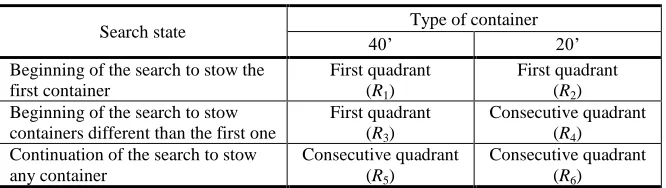
C are tried to assign, and subsequently, this procedure is repeated again to load containers belonging to C_dT. In this procedure, we first select a quadrant with the rules summarized in the Table 1 which are described as follows. If this assignation is the first for any of the two sets of containers, we select the First quadrant (Line 7); this is expressed in Rules R1 and R2. In the next step (Line 8), we choose the first available location to try to assign the container to be positioned. UB2 searches an available location in each quadrant by traversing the tiers, rows and bays orderly. The 40’ containers will be assigned in locations with even bays, while the 20’ containers will be assigned in locations with odd bays. The candidate bays are those that corresponding to the quadrant selected.

When the candidate location has been selected, we must verify that the assignation is feasible, that is, all the constraints involved in the problem must be satisfied. However, if the assignation is unfeasible, we try to allocate the container into a different quadrant. This quadrant is selected depending on the container type. On the one hand, for a 40’ container, UB2 incrementally selects the next quadrant q1, where qrepresents the number of the current quadrant (Rule R5). In the worst case, this search is performed until the last quadrant (the fourth quadrant). If UB2 evaluates all the quadrants and does not stow the current container, this container is not allocated in the containership in this stage. However, when UB2 tries to assign other container of 40’ different than the first one (Line 6), the selection of the quadrant begins again in the first quadrant (Rule R3). If the assignation is unfeasible, then UB2 tries to assign the container in other quadrant by following the previous explanation (Rule R5). On the other hand, for a 20’ container, UB2 tries to assign it in other quadrant according to the order of selection of the quadrants; the selection order is incrementally consecutive (Rule R6). However, when UB2 tries to stow another container of 20’ (Line 6), it selects the consecutive quadrant instead of selecting the first quadrant again (Rule R4).

Table 1. Rules to select quadrants of the containership

Search state Type of container

40’ 20’

Beginning of the search to stow the first container

First quadrant (R1)

First quadrant (R2) Beginning of the search to stow

containers different than the first one

First quadrant (R3)

Consecutive quadrant (R4) Continuation of the search to stow

any container

Consecutive quadrant (R5)

Consecutive quadrant (R6)

Algorithm 3. Pseudocode of UB2.

Phase 1. Preprocessing.

1. Let C'{C₁,C₂,...,C_D} be a partition of C, where each C_d denotes the set of containers having as destination port d and D stands for the number of destination ports.

2. Split each C_d according to the type of containers, that is 20’ and 40’. Thus, obtaining sets C_dT(Twenty) and C_dF(Forty), respectively.

3. Sort each C_dX in decreasing weight order, where X{T,F}.

4. Split the total locations of the containership in four quadrants.

Phase 2. Feasible assignations.

5. For each type of container X{F,T} do:

6. For each destination d, starting from the last one (D) back to 1, assign first containers belonging to C_dX as follows:

7. Select an unexplored quadrant according to established conditions.

8. Select a location of the quadrant previously chosen.

9. If the selected location lS is available, verify the feasibility of stowing container cC_dX into the aforementioned location. If it is feasible, stow c into l. 10. If the container was not assigned, then go to step 7 to try

to assign it in another quadrant. 11. End For

12. End For

Phase 3. Worst-case stowage of unassigned containers.

13. If there are unassigned containers, stow first all the containers in F into the available locations whose loading times are the highest. Then, stow all the containers in T into the remaining locations with the largest loading times.

5

Computational results

In this section, the performance of the proposed bounds is tested. In the following subsections, we describe the test instances, experimental environment and the computational analysis to evaluate the performance.

5.1. Test cases

In order to validate the proposed bounds, we used three sets of instances: A, B and C. The sets A and B have 24 instances each one, while the set C has 10 instances. Each test case (instance) is composed of four characteristic sets:

1) Container sets

2) Containership characteristics 3) Tolerances

4) Loading times

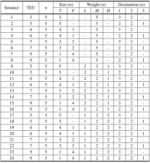
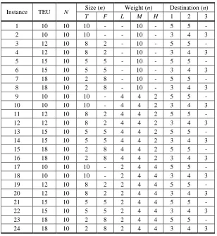
Tables 2, 3 and 4 report the containers characteristics of the sets A, B and C, respectively. Each table shows the total number of containers, expressed in TEU (Twenty-foot Equivalent Unit) and the absolute number (n); the numbers of containers whose type is 20’ (T) and 40’ (F), respectively; the number of containers for three classes of weight (L: low, M: medium, H: high); and the partition of containers by destination. Three classes of weight are considered, namely low (from 5 to 15 tons), medium (from 16 to 25 tons) and high containers (from 26 to 32 tons).

Table 2. Containers for the set of instances A

Instance TEU n Size (n) Weight (n) Destination (n)

T F L M H 1 2 3

1 5 5 5 - - 5 - 3 2 -

2 5 5 5 - - 5 - 2 2 1

3 6 5 4 1 - 5 - 3 2 -

4 6 5 4 1 - 5 - 2 2 1

5 7 5 3 2 - 5 - 3 2 -

6 7 5 3 2 - 5 - 2 2 1

7 9 5 1 4 - 5 - 3 2 -

8 9 5 1 4 - 5 - 2 2 1

9 5 5 5 - 2 2 1 3 2 -

10 5 5 5 - 2 2 1 2 2 1

11 6 5 4 1 2 2 1 3 2 -

12 6 5 4 1 2 2 1 2 2 1

13 7 5 3 2 2 2 1 3 2 -

14 7 5 3 2 2 2 1 2 2 1

15 9 5 1 4 2 2 1 3 2 -

16 9 5 1 4 2 2 1 2 2 1

17 5 5 5 - 1 2 2 3 2 -

18 5 5 5 - 1 2 2 2 2 1

19 6 5 4 1 1 2 2 3 2 -

20 6 5 4 1 1 2 2 2 2 1

21 7 5 3 2 1 2 2 3 2 -

22 7 5 3 2 1 2 2 2 2 1

23 9 5 1 4 1 2 2 3 2 -

Table 3. Containers for the set of instances B

Instance TEU N Size (n) Weight (n) Destination (n)

T F L M H 1 2 3

1 10 10 10 - - 10 - 5 5 -

2 10 10 10 - - 10 - 3 4 3

3 12 10 8 2 - 10 - 5 5 -

4 12 10 8 2 - 10 - 3 4 3

5 15 10 5 5 - 10 - 5 5 -

6 15 10 5 5 - 10 - 3 4 3

7 18 10 2 8 - 10 - 5 5 -

8 18 10 2 8 - 10 - 3 4 3

9 10 10 10 - 4 4 2 5 5 -

10 10 10 10 - 4 4 2 3 4 3

11 12 10 8 2 4 4 2 5 5 -

12 12 10 8 2 4 4 2 3 4 3

13 15 10 5 5 4 4 2 5 5 -

14 15 10 5 5 4 4 2 3 4 3

15 18 10 2 8 4 4 2 5 5 -

16 18 10 2 8 4 4 2 3 4 3

17 10 10 10 - 2 4 4 5 5 -

18 10 10 10 - 2 4 4 3 4 3

19 12 10 8 2 2 4 4 5 5 -

20 12 10 8 2 2 4 4 3 4 3

21 15 10 5 5 2 4 4 5 5 -

22 15 10 5 5 2 4 4 3 4 3

23 18 10 2 8 2 4 4 5 5 -

24 18 10 2 8 2 4 4 3 4 3

Table 4. Containers for the set of instances C

Instance TEU n Type (n) Weight (n) Destination (n)

T F L M H D1 D2 D3

1 69 50 31 19 23 25 2 23 27 0

2 83 60 37 23 26 32 2 27 33 0

3 85 65 45 20 30 33 2 31 34 0

4 88 65 42 23 29 34 2 31 34 0

5 90 70 50 20 31 37 2 30 40 0

6 90 75 60 15 35 38 2 32 43 0

7 93 65 37 28 30 33 2 31 34 0

8 93 70 47 23 29 39 2 32 38 0

9 93 70 47 23 31 36 3 25 20 25 10 94 74 54 20 34 38 2 25 25 24

The tolerances for the set of instances A and B are the following. Maximum horizontal weight tolerance (Q₁) was fixed to 20 tons and maximum cross weight tolerance (Q₂) to 40 tons. The tolerances for the set C are the following. Q₁ was fixed to 18% of the total weight of all the containers to be loaded. While Q₂ was fixed to 9% of the total weight, expressed in tons. Regarding MT, which is the maximum weight tolerance of three containers stack of 20’ was fixed to 45 tons and; MF (the maximum weight tolerance of three containers stack of 40’) was fixed to 66 tons. It is important to point out that MT and MF

were used in all set of instances (A, B and C).

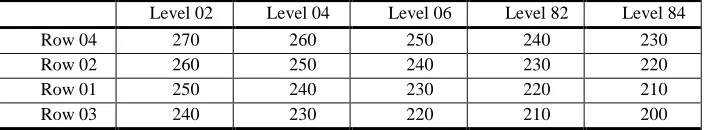
Tables 5, 6, and 7 show the loading times for the containership corresponding to sets of instances A, B and C, respectively. The times are expressed in 1/100 of minute.

Table 5. Loading times for the set of instances A

Level 02 Level 04 Level 82

Row 02 150 144 138

Row 01 144 138 132

Table 6. Loading times for the set of instances B

Level 02 Level 04 Level 82 Level 84

Row 04 156 150 144 138

Row 02 150 144 138 132

Row 01 144 138 132 126

Row 03 138 132 126 120

Table 7. Loading times for the set of instances C

Level 02 Level 04 Level 06 Level 82 Level 84

Row 04 270 260 250 240 230

Row 02 260 250 240 230 220

Row 01 250 240 230 220 210

Row 03 240 230 220 210 200

5.2. Experimental environment

The following configuration corresponds to the experimental conditions:

Software for general purpose: Operating system Microsoft Windows 7 Home Premium; Java programming language, Java Platform, JDK 1.6; and integrated development environment, NetBeans 7.2.

Software for optimization: solver CPLEX 12.5.

Hardware:Computer equipment with processor Intel (R) Core (TM) i5 CPU M430 2.27 GHz and RAM of 4 GB.

5.3. Computational analysis

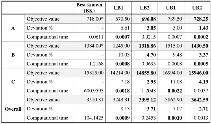
Table 8. Comparison over sets A (24 instances), B (24 instances), C (10 instances) and all the instances (58)

Best known

(BK) LB1 LB2 UB1 UB2

A

Objective value 718.00* 670.50 696.08 739.50 728.25

Deviation % - 6.61 3.05 3.00 1.43

Computational time 0.0611 0.0007 0.0215 0.0007 0.0002

B

Objective value 1384.00* 1245.00 1318.86 1515.00 1430.50

Deviation % - 10.03 4.70 9.48 3.37

Computational time 1.2168 0.0008 0.0695 0.0008 0.0005

C

Objective value 15315.00 14214.00 14855.80 16994.00 15946.00

Deviation % - 7.18 2.95 11.08 4.19

Computational time 600.9595 0.0018 1.2043 0.0022 0.0057

Overall

Objective value 3510.31 3243.31 3395.12 3862.90 3642.59

Deviation % - 8.13 3.71 7.07 2.71

Computational time 104.1425 0.0009 0.2453 0.0010 0.0013

*Average of the optimal solutions

From the experimental results we can observe the following: regarding the lower bounds, LB1 is faster than LB2 by 99.6%. However, LB2 seems to be better in the average quality of solutions for all instances. Specifically, LB2 outperforms LB1 by 4.5% in quality. We can also observe that the percentage of deviation for LB2 is less than that for LB1 by 54.3%. Furthermore, the percentage of deviation for LB1 is approximately 2.2 times greater than that for LB2.

With respect to the upper bounds, it can be seen that UB2 is better than UB1 in two of the attributes. More precisely, UB2 outperforms UB1 by 5.7% and 61.7%, in solution quality and percentage of deviation, respectively. The percentage of deviation for UB1 is approximately 2.6 times greater than that for UB2. Additionally, UB1 is faster than UB2 by 20.8% for all instances.

In order to determine the best combination of lower and upper bounds, we compute the gap, the time and the cost-benefit ratio between every pair of lower bound and upper bound. Table 9 summarizes the comparison of all the combinations. The measures are calculated using the last row (Overall) in Table 8. The first heading in Table 9 shows the gap (%Gap), which is computed by





%GapUBLB UB . The second heading shows the average computing time (Time) that is computed by





Time  , where Time_LB and Time_UB are the average computing time required to compute the lower bound and the upper bound, respectively. Finally, the last heading shows a cost-benefit ratio (Ratio) to consider both the time spent and the quality obtained (1/Gap) by each combination. This ratio is calculated by Ratio1





Table 9. Comparison of all the combinations of lower bounds and upper bounds

%Gap Time Ratio

LB1 and UB1 16.0 0.0010 64.0

LB1 and UB2 11.0 0.0011 82.5

LB2 and UB1 12.1 0.1231 0.7

LB2 and UB2 6.8 0.1233 1.2

6

Conclusions

In this paper the Master Bay Planning Problem (MBPP) was faced. When solving this kind of problems, an important issue is to develop good lower and upper bounds to reduce the search space of optimization algorithms. Therefore, we have proposed two new lower bounds, LB1 and LB2, and two new upper bounds, UB1 and UB2. Heuristics LB1, UB1 and UB2 are deterministic and easy to implement since they are constructed taking into account the problem characteristics. LB1 and UB1 are designed in such a way that their computational effort is low. Although UB2 is a more sophisticated procedure, it only requires a little bit more computational time to be executed. LB2 has good performance with respect to LB1. However, LB2 becomes slower as the size of the instance increases since it is based on a relaxation of the IP formulation.

We tested the performance of all the bounds with three sets of instances. Each lower and upper bound solved all the instances and the results were analyzed by computing the proximity to the best known objective values. The results clearly showed that the best lower bound is LB2 in solution quality and LB1 in computational time. UB2 outperforms UB1 in solution quality whereas UB1 is faster than UB2. When combining the lower bounds with the upper bounds, the best combination is LB2 and UB2 when considering only the Gap. Considering the computational time, the best combination is LB1 and UB1 since they bound each instance in 1 millisecond in average. These results indicate some tendencies which might not be conclusive since the attributes are analyzed independently. In order to consider both attributes together (Gap and Time), we propose to evaluate a cost-benefit ratio for each combination. The result of this analysis indicates that LB1 and UB2 is the best combination of lower bound and upper bound. They achieve the best compromise between quality and time.

Thus, through this research, we allow other researchers to select the best bounds according to their own objectives. For example, some researchers might be more interested in the quality of the solutions rather than the computational time spent or vice versa depending on the problem approached. Nevertheless, there might be some application problems in which the balance between quality and time is required. As a future work, it could be interesting to evaluate the impact of the proposed bounds in optimization algorithms.

References

1. Cruz-Reyes, L., Hernández, P., Melin, P., Huacuja, H. J. F., Mar-Ortiz, J.: Constructive algorithm for a benchmark in ship stowage planning. In: Recent Advances on Hybrid Intelligent Systems. Springer Berlin Heidelberg, 393-408 (2013)

2. Chen, D. S., Batson, R. G., Dang, Y.: Applied integer programming: modeling and solution. John Wiley & Sons (2010)

3. Avriel, M., Penn, M., Shpirer, N.: Container ship stowage problem: complexity and connection to the coloring of circle graphs. Discrete Applied Mathematics, 103(1), 271–279 (2000)

4. Ambrosino, D., Sciomachen, A., Tanfani, E.: A decomposition heuristics for the container ship stowage problem. Journal of Heuristics 12, 211–233 (2006)

5. Ambrosino, D., Sciomachen, A., Tanfani, E.: Stowing a Containership: The master bay plan problem. Transportation Research Part A: Policy and Practice 38 (2), 81–99 (2004)

6. Delgado, A., Jensen, R.M., Janstrup, K., Rose, T.H., Andersen, K.H.: A constraint programming model for fast optimal stowage of container vessel bays. European Journal of Operational Research, 202 (1),251-261(2012)

7. Venkataraman, G., Hu, J., Liu, F.: Integrated placement and skew optimization for rotary clocking. Very Large Scale Integration (VLSI) Systems, IEEE Transactions on, 15(2), 149-158 (2007)

8. Balas, E., Saltzman, M. J.: An algorithm for the three-index assignment problem. Operations Research, 39(1), 150-161 (1991) 9. Cruz-Reyes, Laura, Hernández, P. H., Melin, P., Huacuja, H. J. F., Mar-Ortiz, J., Soberanes, H. J. P., Barbosa, J. J. G. .: A loading

procedure for the containership stowage problem. Recent Advances on Hybrid Approaches for Designing Intelligent Systems. Springer International Publishing, 543-554 (2014)