in the population sciences published by the Max Planck Institute for Demographic Research Doberaner Strasse 114 · D-18057 Rostock · GERMANY www.demographic-research.org
DEMOGRAPHIC RESEARCH
VOLUME 4, ARTICLE 8, PAGES 203-288
PUBLISHED 13 JUNE 2001
www.demographic-research.org/Volumes/Vol4/8/
DOI: 10.4054/DemRes.2001.4.8
A Guide to Global Population Projections
Brian C. O'Neill
Deborah Balk
Melanie Brickman
Markos Ezra
1. Introduction 204
2. Projections and their uses 205
3. Who produces projections? 206
3.1 The United Nations (UN) 207
3.2. The World Bank 208
3.3 The United States Census Bureau (USCB) 208
3.4 The International Institute for Applied Systems
Analysis (IIASA)
209
3.5 The Population Reference Bureau (PRB) 209
4. Projection methodology 210
4.1 The cohort-component method 210
4.2 Alternative methods 213
4.2.1 Time series 213
4.2.2 Microsimulation 214
4.2.3 Structural models 214
4.3 Multistate cohort-component projections 215
4.4 Uncertainty 217
4.4.1 Scenarios 217
4.4.2 Probabilistic projections 219
4.4.2.1 Expert opinion 219
4.4.2.2 Statistical methods 220
4.4.2.3 Historical error analysis 220
4.4.3 Choosing a population projection 221
5. General assumptions 223
5.1 Baseline data 223
5.2 Projecting future fertility 225
5.2.1 Conceptual basis for projections 225
5.2.1.1 Demographic transition theory 225
5.2.1.2 Policies 228
5.2.1.3 Eventual fertility 229
5.2.2 Feedbacks: Environmental change and fertility 232
5.2.3 Current projections 233
5.2.3.1 UN 233
5.2.3.2 IIASA 235
5.2.3.3 U.S. Census Bureau 235
5.2.3.4 Comparison 237
5.3 Projecting future mortality 239
5.3.1 Conceptual basis for projections 239
5.3.1.1 Life expectancy 240
5.3.1.2 New epidemics (HIV/AIDS) 241
5.3.2 Feedbacks: Carrying capacity and health 242
5.3.3 Current projections 245
5.3.3.1 UN 245
5.3.3.2 IIASA 245
5.4.2 Feedbacks: Environmental refugees 252
5.4.3 Current projections 254
5.4.3.1 UN 254
5.4.3.2 IIASA 254
5.4.3.3 U.S. Census Bureau 255
6. Projection outcomes 255
6.1 Population size 255
6.1.1 Regional and national comparison 256
6.1.2 Momentum 258
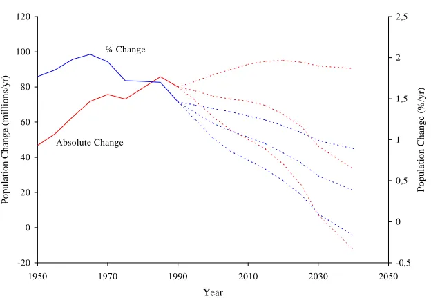
6.1.3 Absolute vs. relative growth 259
6.1.4 Recent UN revisions 250
6.2 Age structure 251
6.3 Distribution 252
6.3.1 Urbanization 252
6.3.2 Regional balance 254
6.4 Accuracy of projections 255
7. Acknowledgments 262
Notes 262
A Guide to Global Population Projections
Brian C. O'Neill 1
Deborah Balk 2
Melanie Brickman 3 Markos Ezra 4
Interdisciplinary studies that draw on long-term, global population projections often make limited use of projection results, due at least in part to the historically opaque nature of the projection process. We present a guide to such projections aimed at researchers and educators who would benefit from putting them to greater use. Drawing on new practices and new thinking on uncertainty, methodology, and the likely future courses of fertility and life expectancy, we discuss who makes projections and how, and the key assumptions upon which they are based. We also compare methodology and recent results from prominent institutions and provide a guide to other sources of demographic information, pointers to projection results, and an entry point to key literature in the field.
1 Watson Institute for International Studies and Center for Environmental Studies, Brown University,
Providence, RI, USA. Email: [email protected], Tel.: 401-863-9916, Fax: 401-863-2192
2 Center for International Earth Science Information Network (CIESIN), Columbia University, Palisades,
NY, USA. Email: [email protected]
3 Center for International Earth Science Information Network (CIESIN), Columbia University, Palisades,
NY, USA. Email: [email protected]
4 Population Studies and Training Center, Brown University, Providence, RI, USA. Email:
1. Introduction
Demographic factors are important components of both the causes of and responses to future economic, environmental, and social change. Interdisciplinary studies of future global change can draw on projected trends in population size and growth rate, age structure, urbanization, and migration, among other variables. Often, however, integration does not proceed far beyond uncritical acceptance of a single projection of future population size. For example, studies of environmental change may use projections simply to scale per capita trends in other factors. Part of the difficulty in making fuller use of projections in such work stems from uncertainties in how demographics, acting in concert with social, economic, and cultural forces, may affect the environment. However, the historically opaque nature of the projection process has presented obstacles as well. How projections are made, the basis for key assumptions, and how projections differ among institutions that produce them has not always been clear to users, making the interpretation of results difficult.
2. Projections and their uses
Population projections (Note 1) differ widely in their geographic coverage, time horizon, types of output, and use. Spatial dimensions can range from local areas (like counties or cities) to the entire world. Local-area projections tend to use shorter time horizons, typically less than 10 years, whereas national and global projections can extend decades into the future, and in some cases more than a century. These longer-term projections typically produce a more limited number of output variables, primarily population broken down by age and sex. In contrast, projections for smaller regions often include other characteristics as well, which might include educational and labor force composition, urban residence, or household type.
The diversity of types of projections is driven by the diversity of users' needs (Lutz et al 1996a). Commercial organizations often use projections for marketing research and generally want a single most likely forecast. They typically want population classified by socioeconomic categories such as income and consumption habits (in addition to age and sex) and by place of residence. Government planners may be concerned with population aging and its potential social and economic impact. They may therefore desire longer-term projections, and want to know more about the health status and living arrangements of the elderly.
The policy community, including advocacy groups, often would like alternatives to a single most likely scenario, including projections that reflect the influence of policy. For example, those concerned with the environmental impacts of population growth may be interested in the potential for reductions in such growth through population-related policies. In addition, they may want to know what the potential effect of environmental feedbacks on growth might be, a topic recently highlighted as underdeveloped by the National Research Council (NRC 2000). Global change researchers often use projections as exogenous inputs to studies on topics such as energy consumption, food supply, and global warming. These studies usually require projections with long time horizons (a century or more) and a range of scenarios rather than a single most likely projection.
institutions produce such projections, but research and practice has been evolving rapidly.
3. Who produces projections?
The earliest systematic global population projection dates to Notestein (1945), although many national level projection efforts began over half a century earlier (see reviews by Dorn 1950 and Hajnal 1955). Since the 1950s, the United Nations (UN) has taken a leadership role in the production of projections and dissemination of their results. Later efforts, most of which continue to date, have been undertaken by three other institutions: the United States Census Bureau (USCB), the World Bank (WB), and the International Institute for Applied Systems Analysis (IIASA). Global long-run population projections tend not to be undertaken by individual researchers. Individual researchers have tended to create projections at the national-level (or below) and at this level have made significant contributions to varying methodologies (see section 4).
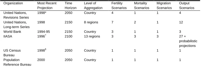
Table 1: Summary of projection characteristics, by key institutions
Organization Most Recent Projection Time Horizon Level of Aggregation Fertility Scenarios Mortality Scenarios Migration Scenarios Output Scenarios United Nations, Revisions Series
1998* 2050 Country 4 1 1 4
United Nations, Long-term Series
1998 2150 8 regions 7 2 1 12
World Bank 1994-95 2150 Country 3 1 1 3 IIASA 1996†
2100 13 regions 3 3 3 27 + probabilistic projections US Census
Bureau
1998§
2050 Country 1 1 1 1
Population Reference Bureau
2000 2050 Country 1 1 1 1
* The UN has recently produced its 2000 Revision, but complete results were not available at the time of this writing.
†
IIASA has recently updated its probabilistic projections, but full documentation is not yet available. Preliminary results are discussed in the main text.
§
In addition to these published projections, the USCB offers more recent projection output (2000) on-line (see: http://www.census.gov/ipc/www/idbsprd.html).
3.1 The United Nations (UN)
Between 1951 and 1998, the United Nations has produced 16 sets of estimates and projections covering all countries and areas of the world. Prior to 1978, new revisions were published approximately every 5 years; since then, they have been published every 2 years. These projections, published in their World Population Prospects series, include four scenarios which differ in their assumptions about future fertility rates: high, medium, and low fertility scenarios, as well as an illustrative scenario in which fertility is held constant at current rates.
addition, another five scenarios illustrate the influence of rising life expectancy on projection outcomes by pairing the first five fertility scenarios with alternative mortality scenarios in which mortality is assumed to remain constant after 2025 or 2050.
3.2 The World Bank
In 1978, the World Bank began producing population projections associated with their annual World Development Report (e.g., World Bank 1984). Projections are made at the country level, and until 1984 results were reported only for 1990, 2000, and the year in which the population became stationary (Note 3). More recent versions of the World
Development Reports contain population projections out to 2000 and 2025, but not the
year at which stationarity is achieved.
From 1984 through 1994-95 the World Bank produced a total of six roughly biennial long-term projections, out to 2150 (the first and last of these are Vu 1984; and Bos et al 1994). Until 1992-93, projections included only one variant. The 1992-93 and 1994-95 projections have a “base-case” and two alternative projections that assume either slow or rapid fertility decline (McNicoll 1992; World Bank, 1994). In additional to global population projections, the World Bank also produced numerous long-range regional projections. Since the 1994-95 projections, the World Bank no longer publishes their projection results although they continue to make long-term projections for internal use (e.g., for pension projects) (E. Bos, pers. communication).
Since 1997, the World Bank has included 40-year (45-year, starting in 2000) projection output as part of their World Development Indicators CD-ROM (cf., WB, 2000). Because the World Bank’s published projections are less than 50 years, we do not consider their projections in detail.
3.3 The United States Census Bureau (USCB)
3.4 The International Institute for Applied Systems Analysis (IIASA)
The Population Project at IIASA first produced a set of long-range global population projections in 1994 (Lutz 1994), and updated those projections in 1996 (Lutz 1996). Projections are made for 13 regions of the world through 2100, and three scenarios for fertility, mortality, and migration are considered. The full set of possible combinations of these assumptions leads to a total of 27 output scenarios, but even this understates the possible total because for a given migration scenario, different scenarios for fertility and mortality in each region can be selected and combined by the user without sacrificing self-consistency (i.e., net migration for the world is always zero). A unique feature of the IIASA projections is that they also provide probabilistic output: that is, the likelihood that population will reach a given size and age structure over the course of the projection period (see section 4). IIASA has recently updated their probabilistic projections, but details were not yet available at the time of this writing.
3.5 The Population Reference Bureau (PRB)
The PRB annually produces a World Population Data Sheet, which contains information such as population counts, fertility and infant mortality rates, doubling time, proportion urban and short population projections out to 2010 and 2025 for all countries in the world. Starting with their 2000 version of the Data Sheet, they have begun projecting population to 2025 and 2050 (PRB 2000). They distribute their output — total population size only, a single scenario — for all countries and select regions, via the web and hard copy.
4. Projection methodology
4.1 The cohort-component method
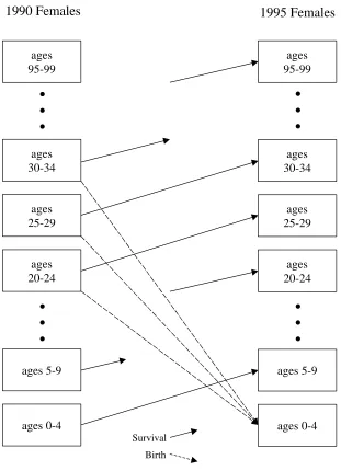
While some projections for individual countries or regions have been made with alternative techniques, all long-term global population projections employ the cohort-component method (Note 4). Initial populations for countries or regions are grouped into cohorts defined by age and sex, and the projection proceeds by updating the population of each age- and sex-specific group according to assumptions about three components of population change: fertility, mortality, and migration. Each cohort survives forward to the next age group according to assumed age-specific mortality rates. Five-year age groups (and five year time steps) are commonly used (although not strictly necessary) for long-range projections (Note 5). As an example, the number of females in a particular population aged 20-25 in 2005 is calculated as the number of females aged 15-20 in 2000 multiplied by the assumed probability of survival for females of that age over the time period 2000-2005. This calculation is made for each age group and for both sexes, and repeated for each time step as the projection proceeds. Migration can be accounted for by applying age- and sex-specific net migration rates to each cohort as well, and ensuring that immigration equals emigration when summed over all regions.
The size of the youngest age group is also affected by the number of births, which is calculated by applying assumed age-specific fertility rates to female cohorts in the reproductive age span (see Figure 1). An assumed sex ratio at birth is used to divide total births into males and females.
Development of this approach was the major innovation in the evolution of projection methodology. It was first proposed by the English economist Edwin Cannan (1895), and was then re-introduced by Whelpton (1936), formalized in mathematical terms by Leslie (1945), and first employed in producing a global population projection by Notestein (1945). Prior to the mid-20th century, the few global population projections that had been made were based on extrapolations of the population growth rate applied to estimates of the total population of the world (Frejka 1981, 1994).
Figure 1: An illustration of one time step of the cohort component method for a female population. (After Cohen 1995, Figure 7.2).
ages
95-99
ages
95-99
ages
30-34
ages
25-29
ages
20-24
ages 5-9
ages 0-4
ages
30-34
ages
25-29
ages
20-24
ages 5-9
ages 0-4
.
.
.
.
.
.
.
.
.
.
.
.
1990 Females
1995 Females
Survival
entirely on the size and age structure at the beginning of the period and the age-specific fertility, mortality, and migration rates over the projection period. Uncertainty in projection outcomes arises not from uncertainty in the formal projection model itself, but from uncertainty in the baseline population data and the assumptions of future trends in vital rates.
The fact that projecting fertility, mortality and migration plays a central role in the cohort-component methodology is considered a strength because it allows demographers to draw on specialized knowledge of each of these components of population change. Institutions therefore normally project trends in vital rates based on expert opinion. Historically, however, it has been difficult to determine precisely how knowledge has been applied to such projections. Assumptions and reasoning have been hidden behind a "veil of secrecy" (Ahlburg and Lutz 1998). For example, while both the UN and the USCB provide general descriptions of their methodology (UN 1999a, 1999d, USCB 1998), neither institution provides a detailed accounting of the reasoning underlying the specific assumptions made for different countries and regions of the world. In general terms, the UN arrives at scenarios for future trends in vital rates through the use of in-house expertise, supplemented by consultation with groups of experts that are occasionally convened to discuss specific topics.
4.2 Alternative methods
4.2.1 Time series
Some national population projections have been made based on analyses of time series of either aggregate population size, or of vital rates. Aggregate time series models do away with the cohort component method entirely. For example, Pearl and Reed (1920), working before the cohort component method had been formalized and widely adopted, sought to apply a simple law of population growth such as the logistic (S-shaped) curve to extrapolate past changes in population size. Leach (1981) re-examined the approach using data from several countries and found it useful in describing historical changes in population size and for short-term projections. Marchetti et al. (1996) found that historical trends in total fertility and life expectancy, as well as population size, are well-approximated by logistic curves. However, in both of these more recent studies it was concluded that the logistic model provides little basis for extending trends into the long-term future. The fundamental difficulty is that a single logistic curve assumes a fixed limit to the variable being modeled, and in human populations those limits can be altered through changes in technology (e.g. changes in agricultural productivity, or health care) or social factors (e.g. changes in family size norms). Thus while a particular curve may fit historical observations, it does not provide any guidance on how the assumed limit may be altered in the future. Furthermore, a logistic function does not allow the direction of change to be reversed. For example, it does not allow for a decreasing population size, or a reversal in the direction of modeled fertility change.
However aggregate time series methods have several drawbacks. For example, confidence intervals quickly become large, limiting their usefulness for longterm projections. In addition, users often desire forecasts not only of total population size, but of age and sex composition as well. Therefore a disaggregated projection might be preferable even if it is no more accurate (Note 6). Perhaps more importantly, aggregate methods do not explicitly take into account the age distribution of a population, which affects the evolution of its size, and also may miss impending changes in the growth rate signaled in advance by changes in fertility or mortality (Lee et al 1995).
4.2.2 Microsimulation
In contrast to the cohort-component method, which treats each cohort as a homogenous group and uses average probabilities of birth, death, and migration, microsimulation treats each individual independently and uses repeated random experiments instead of average probabilities (van Imhoff and Post 1998). This technique simulates life events (marriage, divorce, the birth of children, leaving home, etc.) for each individual, and is usually based on a sample rather than an entire population in order to reduce computational demands; results are then scaled to the size of the total population. A drawback of the microsimulation method is that data requirements can be prohibitive, since probabilities for each life event must be estimated from event-history data. One main advantage of microsimulation is its ability to perform well even with large numbers of "states," or attributes of individuals. In a cohort-component model, the computational requirements for the projection quickly become unmanageable as the number of states increases, since the model must track every possible combination of states. In contrast, a microsimulation model tracks states for each individual in the sample, which is generally a much more manageable task. Since long-term global population projections incorporate only two states (age and sex), microsimulation is unnecessary. However, this method could play a role in studies of the environmental impacts of household consumption, which might require projections with much more detail in household characteristics.
4.2.3 Structural models
relations between demographic and other variables are not generally considered well known enough to quantify reliably (Cohen 1998). The best known example of an attempt to formulate a comprehensive, causal model of demographic processes is the World3 model that served as the basis for the Limits to Growth study in the early 1970s (Meadows et al 1971). The model projected future trends in population, economic growth, and natural resource use, and concluded that global society was likely to collapse in the future due to resource scarcity and environmental degradation. The model assumed fertility and mortality were complex functions of many factors, including population size, birth control effectiveness, health services, life expectancy, income, and industrial output per person. It was strongly criticized for having little empirical or theoretical basis to substantiate the forms used for these and other relationships in the model (e.g., Nordhaus 1973).
Recently, however, several researchers have argued that causal models of more limited scope can contribute usefully to population projections (Sanderson 1998, Ahlburg 1998). Some formal models of fertility, mortality, and migration that include socioeconomic variables (e.g., literacy and female labor-force participation rates) have been shown to produce more accurate forecasts than models that do not explicitly take them into account, and averages of results from the two methods performed better than either approach alone. Combining the results of forecasts produced using a range of different methods may be a source of innovation in future global population projections (especially those requiring greater detail about socioeconomic assumptions), although obstacles remain in selecting which results are of sufficient quality to include in such a procedure.
4.3 Multistate cohort-component projections
Projections that take additional characteristics, or "states," of a population into account are called multistate projections. Multistate projections using the cohort component framework were originally developed in order to account for the place of residence of population members (Rogers 1975) and have since been extended to other dimensions. For example, some multistate projections have taken education level into account since demographic rates are strongly correlated with education levels in many countries, and educational level is often of interest to projection users (Lutz et al 1998a). In some developing countries education level varies strongly with age (e.g., younger cohorts are more educated than their parents), and fertility varies strongly with education (in general, higher education is associated with lower fertility). Thus as time passes, women age into their reproductive years with higher levels of education than the previous members of the reproductive age group, and fertility may be lower than one would project without explicitly taking education into account. In addition, such projections show how the composition of the population by educational level might evolve. For example, building on previous work for specific regions of the world (Goujon 1997, Yousif et al 1996), Lutz and Goujon (submitted) produced the first global population projections by level of education, generating scenarios for 13 world regions to 2030. Results show that while at the global level educational composition changes only slowly and the gap between men and women is likely to persist, outcomes differ widely across regions. For example, due to large investments in education over the past several decades, China is likely to see the percentage of women over age 15 with some secondary education rise from 35 to at least 60. On the other hand, South Asia (mainly India) is unlikely to see the current proportion of 15% rise beyond 25% even under extremely optimistic assumptions.
A second example of multistate projections is the projection of households in addition to population. Van Imhoff and Keilman (1991) developed a multistate model that they applied to projecting households in the Netherlands; it has subsequently been applied to many other situations. More recently, Zeng et al (1998) developed a model that includes marital status (including cohabitation), parity (number of children ever born), number of children living at home, coresidence, and rural or urban residence. These models allows investigation of how changes in demographic factors such as marriage rates or the age at which children leave home can affect not only fertility and population growth, but also changes in the numbers, size distribution, and composition of households. This may be particularly relevant to energy and environment researchers, since household characteristics may be a key determinant of energy demand (O'Neill and Chen, submitted; MacKellar et al 1995).
urban versus rural population growth, which is not only an output of interest but also a significant source of heterogeneity in fertility and mortality. As emphasis on human capital and investment in education grows, more comprehensive projections incorporating education may be made as well.
4.4 Uncertainty
Accurately characterizing the uncertainty associated with a population projection is critical to ensuring that it is used appropriately. Many studies of global environmental change, for example, rely on a projection assumed to be the “most likely” outcome, and for this reason it seems widely agreed that it is important to provide users with such a projection. However, while it seems equally important to provide users with an indication of the uncertainty associated with the most likely projection, there is no generally accepted approach to characterizing this uncertainty, and in some cases (for example the projections of the U.S. Census Bureau) it is not done at all. The recent report of the U.S. National Research Council (NRC 2000) concluded that insufficient attention has been given to this issue by agencies making projections, and marks it as a priority for research. Different approaches to characterizing uncertainty can be grouped into two main classes: scenarios and probabilistic projections.
4.4.1 Scenarios
The most common approach is to present alternative scenarios that assume higher or lower vital rates than in the medium or central scenario. Terminology regarding alternative projections can be confusing. For example, the UN uses the term "variant" to describe alternative projections in its 1998 Revision, but uses "scenario" to describe alternative projections in its long-range projections. Lutz et al (1998b) note that the term "variant" is often used to define a population projection in which the underlying demographic rates are purely hypothetical and are not assumed to be dependent on external factors such as socioeconomic conditions. In contrast, the term "scenario," which IIASA uses to describe its projections, is defined as a consistent story in which fertility, mortality, and migration assumptions are embedded to provide a comprehensive picture of what the future might be. For simplicity, we call all sets of alternative projections scenarios, with the understanding that the story behind each scenario may be more or less well defined.
independent scenarios rather than confidence intervals around a most likely projection. These alternative projections can be used in building up more comprehensive scenarios that may include many other components such as economic growth, technological development, and greenhouse gas emissions (Gaffin 1998).
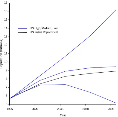
However, the approach also has several weaknesses. The most important is that if no specific level of uncertainty is associated with the alternatives, it is not possible for users to interpret the precise meaning of the ranges presented. For example, the UN long-range projections include a high and low scenario in which fertility rates eventually become constant at about half a birth per woman higher or lower than in the medium scenario. Because these scenarios produce a global population that doubles or is halved every 77 years, the UN assumes that these projections are "unsustainable over the very long run" (UN 1999a, xiii), presumably because they would eventually lead to extinction or to implausible crowding. It therefore produces intermediate scenarios with more moderate rates of growth or decline and concludes that future demographic rates "will very likely be bound by these (intermediate) scenarios if sustainability is to be maintained" (UN 1999a, xiii). However, despite the arguments ruling out population collapse or sustained rapid exponential growth, no other qualitative or quantitative probability is attached to any of the scenarios, nor is any set of socioeconomic conditions defined under which high or low population growth would be likely to occur.
Another problem with the scenario approach is that the choice of certain values for some assumptions may mean that choices for others are unreasonable. For example, the UN scenarios account for possible variations in fertility paths, but not for variations in future migration or mortality (except for a constant mortality case used to demonstrate the relative importance of mortality change to future population growth). On the one hand this approach simplifies interpretation of differences between projection results, which clearly demonstrate sensitivity to fertility assumptions alone. It also can be defended on the grounds that fertility has a larger influence on future population size and growth rates than either migration or mortality. On the other hand it has been criticized on the grounds that it misrepresents plausible future population paths because the conditions that are likely to be associated with lower fertility in developing regions are also likely to be associated with lower mortality (and, similarly, higher fertility is likely to be associated with higher mortality). The IIASA projections provide scenarios in which each vital rate is varied individually, but also provide scenarios in which fertility and mortality are varied jointly.
"canceling" would occur: some regions would follow paths higher than the central assumption while others followed lower paths, reducing the spread of future plausible paths. Both the UN and IIASA scenarios are subject to this weakness, although IIASA scenarios are provided at the regional level in such a way that users can choose to combine regional results from different scenarios and still maintain a self-consistent global population path (Note 7).
Finally, high and low scenarios intended to bracket the range of possible future population sizes will not necessarily also bracket the range of possible age structures or other demographic variables (Lee 1998). For example, although high population growth is generally associated with a young age structure, a path intended to produce the largest population will not produce the youngest one. Population grows fastest when fertility is high and life expectancy is long, but the youngest age structure is produced when fertility is high and life expectancy is short. Thus the scenario approach does not accurately reflect relative uncertainties in different demographic dimensions.
4.4.2 Probabilistic projections
An alternative to scenarios as a means of communicating uncertainty is to explicitly account for uncertainty in projected trends of fertility, mortality, and migration, and derive the resulting probability distributions for projected population size and age structure. There have been three main bases for determining the probabilities associated with vital rates: expert opinion, statistical analysis, and analysis of errors in past projections.
4.4.2.1 Expert opinion
Among the institutions providing long-term global population projections, only IIASA provides probabilistic projections. The IIASA methodology is based on asking a group of interacting experts to give a likely range for future vital rates, where "likely" is defined to be a confidence interval of roughly 90% (Lutz 1996, Lutz et al 1998b). Combining subjective probability distributions from a number of experts guards against individual bias, and IIASA demographers argue that a strength of the method is that it may be possible to capture structural change and unexpected events that other approaches might miss. In addition, in areas where data on historical trends are sparse, there may be no better alternative to producing probabilistic projections.
future trends. Lee (1998) questions whether experts can meaningfully distinguish between different confidence levels they may place on estimates of future vital rates. He also argues that the method excludes the possibility of fluctuations in vital rates that deviate from a general trend, which could underestimate uncertainty in outcomes. For example, there are no scenarios in which fertility starts out high, but ends up low, nor any scenarios with baby booms or busts. In addition, the possibility of capturing the potential for structural change may not be unique to the expert opinion approach; probabilistic projections based formally on errors from past projections implicitly contain information on past structural changes, such as world wars, the baby boom, the spread of modern contraception, the introduction of antibiotics, etc. (Lee 1998).
4.4.2.2 Statistical methods
Statistical analysis of historical time series data can be used either to project population size directly or to generate probability distributions for population size or vital rates. Lee (1998) argues that, unlike methods based purely on expert opinion, these methods are capable of producing internally consistent probability distributions. While statistical methods also employ expert judgment, the mix of subjective and objective methodology is tilted more toward objective methods than is the expert-based method used in the IIASA projections. These methods have been applied only to some national projections (e.g., Lee and Tuljapurkar 1994, Alho 1998), but not to global projections, so they are not discussed further here. However they may be a source of further innovation in long-term global projections.
4.4.2.3 Historical error analysis
projection at a pace based on past experience, and correlations in errors between countries or regions and over time can be accounted for. As an illustration, if large projection errors in some countries at a particular time have generally been associated with large errors in previous periods, or in neighboring countries, a statistical model based on historical experience can capture this tendency.
The results of the NRC uncertainty analysis showed that, averaged across 13 large countries, the 95-percent confidence intervals based on historical error analysis were more than twice as large as the range defined by the UN high and low scenarios, in both the short term and after 50 years. At a more aggregate level, this difference declined: averaged across 10 world regions, the 95-percent confidence intervals in a 50-year projection were about 40% larger than the UN high-low range. At the global level, the estimated 95 percent confidence interval was somewhat narrower than the UN high-low range. This pattern in the comparison of the two ranges occurs because the NRC analysis takes into account the cancellation of errors at higher levels of aggregation; that is, projected regional population sizes are less uncertain than projected sizes of the countries that make them up because over- and under-estimates for countries will cancel to some extent at the regional level. The same holds true in comparing uncertainty at the global and regional level. The UN methodology, based on the scenario approach, cannot take this phenomenon into account, and the high-low ranges are similar at all levels of aggregation. The NRC analysis also concludes that global population size is extremely unlikely to begin declining before 2050, even though it does so in the UN low scenario, and that the probability that the UN median scenario significantly underestimates future population size, while low, is higher than the probability that it is a significant overestimate.
4.4.3 Choosing a population projection
Users face a number of choices in selecting demographic inputs for their analyses. The considerations involved in such choices are many and varied, and depend on the nature of each application. While it is beyond the scope of this paper to discuss the larger question of how best to integrate demographic projections into integrated analyses, we offer some suggestions that follow directly from the discussion of different treatments of uncertainty in this section.
If it is decided that scenarios will be used, the choice of which population scenarios or set of scenarios to use should take into account the assumptions on which they were based and their sources of uncertainty. For example, to avoid internal inconsistencies, a population projection based on an assumption of slow economic development and incremental health improvements should not be used in a larger analysis that is based on a different set of underlying assumptions. This task is made somewhat difficult by the limited description of underlying assumptions for some population projections, but should be kept in mind. Users should also keep in mind that the range of uncertainty in particular demographic variables differs across a given set of scenarios. Recognizing that the choice of one set of high and low scenarios may bracket plausible population size ranges, but may not bound the set of plausible age distributions, would be essential for researchers investigating problems with both size-and age-sensitive characteristics. A relevant example is the analysis of future pension systems.
Probabilistic projections are attractive to particular applications, but can also inform analyses that are explicitly non-probabilistic. For example, some researchers exploring future scenarios of energy use and greenhouse gas emissions have taken probabilistic approaches and in the past have relied on deriving their own probability distributions for demographic parameters (e.g., Fankhauser 1994). This kind of work could benefit from the recent developments in probabilistic population projections. So, too, could analyses that explicitly avoid probabilistic interpretations. For example, the Intergovernmental Panel on Climate Change (IPCC) recently produced an updated set of scenarios for future greenhouse gas emissions (Nakicenovic et al 2000), with each scenario corresponding to one of four "storylines" regarding broad social, economic, and demographic development patterns. A wide range of input variables and resulting emissions paths are covered, but all scenarios are considered equally sound and interpretation of likelihood is left up to the user. In this case, users might draw on probability distributions of demographic projections to help judge how likely the particular demographic scenario used as a driving force in the IPCC scenarios might be, and therefore how likely the resulting emissions path itself might be.
probabilistic projections taking specific assumptions about determining factors into account, in practice users generally must rely on unconditional projections. With no way to adjust the distributions of output to account for different assumptions about underlying factors, users generally rely on alternative scenarios and must make their own judgment as to what scenario demographers had in mind when producing it and how well it matches their own assumptions. While it is unrealistic to expect agencies to produce conditional projections, better descriptions of the assumptions underlying scenarios or probability distributions might aid users in adapting them to their own needs.
Finally, in many cases it would be beneficial to include demographers on an interdisciplinary research team who can produce projections that are custom-designed for the question at hand. While this is not always feasible, where it is it would have the potential to greatly improve the self-consistency and rigor of the analysis.
5. General assumptions
The mechanics of projecting population growth from base year data and assumed future trends of fertility, mortality, and migration are straightforward and, except for methods of communicating uncertainty, essentially identical across institutions. The real challenge in projecting population lies in accurately determining the characteristics of the initial population (size, age structure, and vital rates) and in projecting future trends in vital rates, although it should be kept in mind that these two undertakings differ in a fundamental way: the characteristics of the initial population can be known with reasonable accuracy, given enough effort, while future trends in vital rates are unknowable. It is, in fact, for this reason that the methods for expressing uncertainty discussed in section 4.4 were developed. All projections of fertility, mortality and migration used in producing global population projections are based in some manner on expert opinion informed by current conditions, past trends, and theories about the determinants of changes in vital rates.
5.1 Baseline data
performed periodically in most countries of the world. In countries where census data is nonexistent or considered inaccurate, data from sample surveys are often used.
The United Nations Population Division produces the most widely used compilation of current and past estimates of population size, age structure, and vital rates based on these primary sources, and obtaining data and evaluating its quality and consistency makes up the bulk of the Division's efforts on demographic matters (Zlotnik, pers. comm.). It must be ensured, for example, that past trends of vital rates are consistent with past estimates of population size and age structure. In developed countries, detailed data on fertility and mortality is usually available, along with reliable periodic census counts. These can be combined to produce a relatively consistent picture of historical population change in these areas. However, even here data on international migration is often inadequate, and complete consistency between vital rates and population change is often achieved by assigning to net migration the residual estimate (Zlotnik 1999a).
Estimations for less developed countries are more difficult due to scarce and sometimes unreliable data. Often indirect estimation techniques must be used, occasionally by inferring rates and levels from other countries in the same region with similar socio-economic characteristics. However, over the past 20 years data collection efforts have increased substantially, and for the UN 1998 revision, 83 percent of all countries or areas had post-1985 census data available on population size and age structure (Zlotnik 1999a). Data on vital rates are often derived from surveys and are more problematic. Information on fertility and child mortality is generally more available than information on adult mortality. For example, countries accounting for about 5 percent of global population lacked data more recent than 1990 on fertility and child mortality. In contrast, countries accounting for 40% of global population lacked data from the 1990s on adult mortality (Zlotnik 1999a). This not only makes the estimation and projection of mortality trends difficult, but, coupled with unreliable census data, makes estimation of the baseline age and sex structure of the population difficult as well.
IIASA used baseline data on population size, total fertility rates, and life expectancies from the Population Reference Bureau's 1995 World Population Data Sheet (see PRB 2000 for the most recent version), combined with age distributions of population and vital rates from the UN 1994 Revision (Lutz et al 1996b). The Population Reference Bureau bases its estimates on the work of the UN, and independent consideration of other sources including official country statistics, the Council of Europe, and the U.S. Census Bureau.
5.2 Projecting future fertility
In the long run, the level of fertility has the greatest effect on population growth because of its multiplier effect: additional children born today will have additional children in the future. Fertility projections are made by projecting the course of the total fertility rate (TFR) over time, and translating this total fertility rate into age-specific fertility rates. In general, the projection of TFR is divided into assumptions regarding a level at which fertility eventually becomes constant in the country or region, and the path taken from current to eventual levels. Once fertility reaches its eventual level, assuming mortality and migration rates are also fixed, the population will eventually reach a stable age structure and constant growth rate. If the eventual fertility level is at replacement level and net migration is zero, the growth rate will eventually be zero − that is, the population will not only be stable, but stationary as well. Both the projected pace of fertility decline and the assumed eventual fertility level are important to determining trends in population size and age structure. The two factors also interact: the lower the assumed eventual fertility level, the more important the pace of fertility decline becomes to projected population size (O'Neill et al 1999).
5.2.1 Conceptual basis for projections
5.2.1.1 Demographic transition theory
The concept of demographic transition is a generalization of the sequence of events observed over the past two centuries in the more developed countries (MDCs). While different societies experienced the transition in different ways, in broad outline these societies have gradually shifted from small, slowly growing populations with high mortality and high fertility to large, slowly growing populations with low mortality and low fertility (Knodel and van de Walle 1979). During the transition itself, population growth accelerates because the decline in death rates precedes the decline in birth rates.
Empirical evidence from all parts of the world overwhelmingly confirms the relevance of the concept of demographic transition to LDCs. The transition is well advanced in all regions except sub-Saharan Africa, and even here the beginnings of a fertility decline are becoming apparent. In several countries such as China, Taiwan, and Korea, fertility is already at sub-replacement levels. In many other countries in Southeast Asia and Latin America, fertility has fallen to levels seen just a few decades ago in MDCs.
The biggest difference between the transition in MDCs and LDCs has been the speed of the mortality decline. In Europe, North America, and Japan, mortality fell slowly for two centuries as food supply stabilized, housing and sanitation improved, and progress in medicine was made. In contrast, mortality in LDCs fell over the course of just a few decades after World War II as Western medical and public health technology and practice spread to these regions. One result is that LDC populations are growing much faster than did the populations of MDCs at a comparable stage of their own transition.
The earliest attempts to explain the demographic transition cited industrialization and urbanization as the ultimate driving force (Thompson 1930, Davis 1945, Notestein 1945). According to this "classical" transition theory, economic modernization leads to improvements in health and nutrition that decrease mortality. Modernization also drives changes in economic and social conditions that make children costly to raise and reduce the benefits of large families. Eventually, this leads to lower fertility; fertility decline lags mortality decline because cultural norms regarding reproduction are difficult to change while improvements in mortality meet little resistance.
investments in education and health, while increases in women's labor force participation and wages increase the opportunity costs of raising children. In addition, some of the economic benefits parents may derive from children, such as household labor, income, and old age security, decline as a result of the development process. Thus, as the net cost of children rises, demand falls.
This framework has been extended and made more flexible by taking into account sociological aspects. Easterlin (1969, 1975) added supply factors (environmental and cultural effects on fertility in the absence of regulation) and costs (including the psychic, social, and monetary costs of fertility regulation) to the focus on demand.
Other explanations have given much more weight to sociological over economic factors. For example, Ryder (1983) argued that reproductive decisions are not based strictly on a rational weighting of the consequences of childbearing, but are strongly influenced by cultural and normative contexts. Caldwell (1982) elaborated a theory that identified a shift away from extended family structures toward the child-centered nuclear family as the cause of a reversal in the flow of wealth (money, goods, services, and guarantees against risk) from children to parents typical in pre-transition societies to a flow benefiting children. As children displace parents as beneficiaries of the family, fertility falls. The shift in family structure could be triggered by economic changes, but also by the spread of new ideas.
Other researchers have emphasized the role of cultural over socio-economic factors. Based on analyses of the fertility transition in Western Europe, Lesthaeghe (1983) argued that differences in fertility across societies were largely due to differences in religious beliefs and the degree of secularism, materialism and individuation. Cleland and Wilson (1987) concluded that ideational change in general, and the spread of new ideas about the feasibility and acceptability of birth control in particular, was a key driver in fertility decline and likely more important than changes in economic conditions. Bongaarts and Watkins (1996) demonstrated that diffusion of ideas and information about limiting fertility is important. They showed that fertility transitions typically start in leader countries where development levels are relatively high, and then spread to other countries in the region, often before they have achieved the same level of development.
particular circumstances remains an elusive goal (NRC 2000, Oppenheim Mason 1997, Kirk 1996, Hirschman 1994).
Although the fact that demographic transition has occurred under so many different conditions and has likely been driven by multiple causes complicates study of the subject, in one sense it can be considered a strength where projections are concerned. It implies that transition is probably inevitable, so that the task of projecting future fertility in high fertility countries is to anticipate not so much whether countries will experience this phenomena, but when, how fast, and to what eventual end state.
5.2.1.2 Policies
The role of population policies in the decline of fertility in developing countries over the past several decades and by extension their potential role in future fertility trends is a matter of some debate. Implementation of family planning programs has been the main policy tool in the past (Note 8), and there are two main points of view on their effectiveness.
Proponents argue that programs have had a substantial effect on fertility primarily by reducing "unwanted fertility" (births that occur after a woman has reached her desired family size) below what it otherwise would have been (Potts 2000). The conventional justification for facilitating this reduction is based on survey data indicating that many women report wanting to avoid pregnancy but do not use contraception. Family planning programs therefore help meet this "unmet need" for contraception by assisting users in overcoming obstacles to contraceptive use, which can include limited access to services, lack of knowledge, fear of side effects, disapproval of families and others, and high cost (Bongaarts and Bruce 1995).
In contrast, Pritchett (1994a, 1994b) has argued that unmet need is much smaller than commonly assumed, and that fertility decline is driven primarily by declining desired fertility (that is, a reduction in the number of children women actually want) rather than a reduction in unwanted fertility. This conclusion is based on the high correlation between total and desired fertility, and the lack of correlation between total and unwanted fertility. He argues that because low fertility countries have low desired fertility, but not especially low unwanted fertility, the fertility decline must have been driven by reductions in desired fertility, not by reduced unwanted childbearing. He also argues that family planning programs have had an insignificant historical effect on fertility.
probably less than commonly cited by advocates of family planning programs, since these estimates include need for contraception for spacing children and meeting that need is unlikely to have a substantial effect on fertility. He also concludes that the effect of programs on unwanted fertility is likely substantial; the critics' view is based on a misinterpretation of the lack of correlation between total and unwanted fertility, which clearly exists but is not inconsistent with effective family planning programs. And finally, he argues that historically programs have in fact had a substantial effect on fertility: an estimated 43 percent of the fertility decline between the early 1960s and late 1980s was due to program interventions.
Future change in fertility will also depend on the extent and effectiveness of future policy. At the 1994 International Conference on Population and Development (ICPD) in Cairo, 179 countries agreed to a Program of Action that marked a fundamental shift in the motivation for population-related policies away from demographic targets and toward a new focus on individual well being. The Cairo program set a number of goals for 2015 that reflected this perspective, among them universal access to comprehensive reproductive health services (including, but not limited to, family planning); reductions in infant, child, and maternal mortality; and universal access to primary education, with an emphasis on closing the "gender gap" between girls and boys. Although these goals are not primarily motivated by their potential effect on demographic trends, achieving them would likely lead to lower fertility. Bongaarts (1994) estimated that eliminating unwanted fertility in developing countries would reduce population in 2100 by about 2 billion, and lowering high desired family size, which could be achieved in part through the measures advocated in the Program of Action, would reduce population by an additional billion.
In the global projections discussed here, population policy efforts and effectiveness are implicitly accounted for, but do not explicitly enter the projection process. Although program effort and effectiveness can be quantified (Ross and Mauldin 1996), quantifying their influence on fertility remains difficult. For example, Mauldin and Ross (1994) took program effort into consideration in their short-term projections for 37 LDCs, but only in establishing uncertainty, not in the fertility projections themselves.
5.2.1.3 Eventual fertility
grappling with the question of future fertility trends in countries that have already completed the transition to low fertility.
Traditionally, long-term projections have assumed that fertility in all countries would eventually stabilize at replacement level, leading to a stationary population. There are two general arguments in favor of this assumption. First, replacement level fertility may be seen not as the most likely outcome, but as a mathematically convenient benchmark which prevents population from steadily growing or declining (UN 1999a). Second, it has been supported on the basis of a systems view which holds that demographic rates of a population are not just the sum of individual behavior, but also reflect the tendency of the demographic system to maintain itself (Vishnevsky 1991). This view sees the falling mortality rates that mark the onset of the demographic transition as a perturbation of a system in homeostasis; birth rates fall as the system inevitably re-establishes balance between the two rates, and fertility seeks replacement level in order to preserve the system. Some researchers have speculated that fertility could be stimulated to rise to replacement level in currently low-fertility countries by a wide range of factors, including pronatalist government policies, increased nationalism, a renewed emphasis on traditional roles for women, or a shift away from materialist values (Day 1995).
However, the return to replacement fertility has been strongly criticized as an assumed magnetic force without empirical support (Demeny 1997, Westoff 1991, Lee 1991). Total fertility has been below replacement level in 20 European countries for at least two decades, and it is currently below 1.5 children per woman in 21 European countries (UN 1999c). In large parts of several European countries (e.g. Eastern Germany, Northern Italy, and the most urbanized regions of the Russian Federation), fertility has been at or below 1.0 (UN 1997b). Several LDCs have reached subreplacement level fertility as well (e.g., China, Thailand, and North and South Korea).
this would leave room in principle for considerable further decline, but it remains unclear whether this limit will be relevant to future fertility trends.
Unfortunately, while current trends and some plausible explanations may suggest continued low future fertility, there is no compelling and quantifiable theory of reproductive behavior in low-fertility societies. Although fertility typically continues to fall after reaching replacement level, there is no clear pattern to subsequent fertility trends. In some countries, fertility falls quickly to very low levels, in others it has made a more gradual decline, in some such as the U.S. and Sweden it has declined well below replacement level and then risen nearly to replacement level again (although Sweden has recently seen another rapid decline) (UN 1997b).
One argument against assuming that total fertility will remain very low in these countries is that because TFR is a period measure, it is affected by changes in the timing of births even if the actual number of births women experience over their lifetime does not change. Since the mean age of childbearing has been increasing in many industrialized countries over the past several decades, part of the decline in TFR has been due to this timing effect and not to a change in the completed fertility of women. Bongaarts and Feeney (1998) therefore argue that TFR is likely to increase in the future once the mean age of childbearing stops rising, as happened in the 1980s in the United States when fertility rose to its current value just below replacement level. An additional argument against continued very low fertility is that in surveys conducted in much of Europe women consistently say they want about 2 children (Bongaarts 1999). There are many reasons why women may fail to reach this target (e.g. competing career plans, divorce, infertility), but this finding suggests that fertility is unlikely to remain extremely low, especially if societies made it easier for women to combine careers and childbearing.
However, it may be unlikely that TFR in European countries will return to near replacement level, even after postponement of childbearing has ceased. This will depend in part on the extent to which younger women who are currently postponing births will recuperate some of this delayed fertility at older ages, which will influence their cohort fertility (Lesthaeghe and Willems 1999). Cohort fertility was already below replacement level in most European countries for women born between 1945 and 1960 (the most recent cohorts for which reliable estimates of completed fertility can be made) (UN 1997a).
(1962) for which it can safely be estimated. The USCB also assumes that eventual fertility will be below replacement level in many countries. It projects that currently high fertility countries will experience a decline to, or slightly below, replacement level. Other countries generally converge to levels between 1.7 and 2.0.
5.2.2 Feedbacks: Environmental change and fertility
Environmental change has had a historically important effect on various demographic rates, including fertility. For example, Galloway (1986) found that warmer than average periods in middle latitudes were associated with above average population levels, and vice-versa. The suggested mechanism was climatic influence on agricultural output and food supply per capita. Data from 16th and 17th century England show that during cool periods, grain yield, fertility, life expectancy, and population growth declined, while the average age at marriage and net out migration increased. Similarly, analysis of data from China and western Europe between the 13th and 19th century indicates that warmer temperatures have been linked to increases in population growth rates.
Links between environmental change, agriculture, and fertility can be mediated by a number of factors. Men may leave the community to seek work in adjoining agricultural regions or in cities (Lee 1990, Hill 1989). Marriages may be delayed because couples lack financial assets. Expectations and the incremental nature of many crises also play a role; for example, Dyson (1991) found an anticipatory demographic response in South Asia, where famines were preceded by extended periods of worsening adversity during which fertility declined. Caldwell et al. (1986) found that stress resulting from the 1980-83 South Indian Drought was associated with a preference for fewer but more educated children.
Ezra (1997) argued that the growing environmental stress and persistent food insecurity endured by Ethiopian communities over the past two decades stimulated changes in the demographic behaviors and attitudes of farming communities. He observed preferences for later age at marriage and smaller family size, a significant increase in acceptance rates of family planning services, actual reductions in fertility, increased migration (particularly of the youth) out of the communities, and the tendency by many farmers to be involved in non-farm income generating activities. It is argued that demographic transition is faster in ecologically degraded communities than in relatively stable ones.
potential for policy to mediate between environmental stress and demographic responses. Currently, no long-term projections explicitly take into account environmental feedbacks on fertility. However, in IIASA's probabilistic projections, the small probability of significant effects are implicitly included in the tails of the fertility distribution (Lutz et al 1996b).
5.2.3 Current projections
5.2.3.1 UN∗
Historically, the medium projection in UN Revisions (which extend to 2050) has incorporated the assumption of universal convergence to replacement level fertility, with somewhat higher and lower levels assumed in the high and low variants. Recently, this approach was abandoned for countries in which fertility is currently below 2.1 (UN 1999d). This change in practice has been based on the observation that the number of countries with below-replacement fertility is large and increasing. By 1995, 44 percent of the world population lived in countries where fertility was at or below replacement level, including several countries in the developing world such as China, North and South Korea, and Thailand. In many of these countries low fertility has persisted for a decade or two. Furthermore, in more than 20 countries, including Italy, Spain, and Germany, fertility has fallen below 1.5 births per woman.
As a result, the medium variant of the 1998 Revision assumes that fertility in countries where it is below 2.1 in 1990-95 will remain below replacement level until 2050. Low fertility countries are divided into two groups: those with fertility in 1990-95 between 1.5 and 2.1, and those with fertility below 1.5. In the first group, fertility is projected to rise to 1.9, and in the second to 1.7, and remain constant thereafter (Note 9). However, in countries with fertility above 2.1 children per woman in 1990-95, the UN maintains its historical assumption that fertility will undergo a smooth decline to replacement level and remain constant thereafter.
The pace of fertility decline for currently high fertility countries is determined by setting a period in which fertility is assumed to reach its eventual level. This determination is made based mainly on the current level of and recent trends in fertility in each country, and a comparison to other countries with similar conditions. The choice of target year has changed little in recent UN Revisions. In currently low fertility countries, data more recent than the base period (1990-95) was used to extend fertility
trends to the 2000-05 period. They were subsequently assumed to change at a constant rate until reaching their ultimate level.
In the high and low scenarios, fertility in countries currently above replacement level was assumed to eventually stabilize at half a birth per woman above and below replacement, respectively. Fertility in countries currently below replacement level was assumed to stabilize at 0.4 births per woman above and below the level it achieved in the medium variant, respectively (Note 10). The pace of fertility change was adjusted so that currently high-fertility countries reached ultimate fertility levels in the same target period as in the medium variant. In low fertility countries, the pace of fertility change was held constant at a slightly greater rate than in the medium variant.
Once total fertility rates were determined for all countries in all periods, they were translated to age specific fertility rates. In countries where fertility is currently below replacement level, age specific rates are generally held constant. In currently high-fertility countries, age patterns are determined by interpolating between the estimated current schedule, and one of three model schedules (UN 1999d) for countries that have completed a fertility transition.
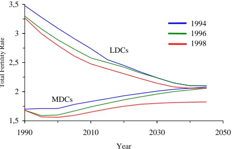
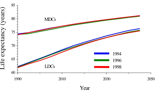
The UN has revised its estimates of current fertility and projections of future fertility over the past several projection cycles. Figure 2 shows projected fertility for MDCs and LDCs for the 1990-2050 period for the UN 1994, 1996, and 1998 Revisions. In 1996, the estimate of LDC fertility in 1990-95 was 3.3, nearly 0.2 births per woman less than the medium variant projection made in 1994 (which used 1985-1990 as the base period), and slightly less than even the 1994 low variant. This revision also lowered projected fertility over the next several decades. Between 1996 and 1998, the base period TFR was revised only slightly, but projected fertility was lowered further over nearly the entire projection horizon. The figure also shows that expectations for future fertility in MDCs have been lowered as well, particularly in the 1998 revision which discarded the assumption of an eventual rise to replacement level in these countries. The net differences for projected population totals in 2050 amount to more than 1 billion: projected population in 2050 dropped from about 10 billion in 1994 to less than 9 billion in 1998.
provide a benchmark scenario in which population ultimately stabilizes, not because it is judged to be the most likely scenario. The projection is described as representing "a conceptual dividing line between long-range future population increase and long-range population decline" (UN 1999a, 34).
Figure 2: Total fertility rate for MDCs and LDCs according to the UN medium
variant in 1994, 1996, and 1998.
5.2.3.2 IIASA∗
IIASA fertility scenarios are based on expert opinion on possible fertility levels in the period 2030-2035. Based on recent experience and the belief that the demographic transition is almost certain to continue, it is assumed that fertility in LDCs will continue to decline. Thus, even in the high scenario, which is based on the possibility that fertility transition is retarded or stalled, fertility in the period 2030-35 is projected to be lower than it is today. One exception is China, where the high variant assumes that fertility rises from 2.0 to 3.0, based on the possibility that the country's one-child policy could be relaxed and fertility might rise as a result. The second exception is Latin America, where it is assumed that fertility stalls in the region as a whole at 3.0 since there is evidence that such a stall has occurred in particular countries due to heterogeneous populations in which some segments are well advanced in the demographic transition while others have hardly started it.
∗ Based on Lutz et al 1996b, Lutz 1995
1,5 2 2,5 3 3,5
1990 2010 2030 2050
Year
Total Fertility Rate
MDCs
LDCs
Low-variant assumptions imply that fertility decline in LDCs, as has been the experience in MDCs, does not stop at a TFR of 2.1 but continues to decline, carrying countries into the range of sub-replacement fertility. The Central assumptions, derived by averaging High and Low variants, are assumed to represent the most likely case and result in slightly above replacement-level fertility in 2030-2035 in most LDC regions − substantially so in sub-Saharan Africa.
In MDCs, the IIASA high scenario assumes a return to replacement level fertility (or slightly above) by 2030-35 (Note 11). This scenario is taken to be representative of the systems view of fertility which argues for an inherent tendency of demographic systems to maintain themselves. The low scenario projects a fertility level of 1.4 in North America and 1.3 in the other developed regions, with central variants obtained by averaging high and low assumptions.
Fertility assumptions for all regions were extended into the future by assuming that in 2080-85, TFR would lie in the range 1.7 - 2.1 in the central scenario, depending on the population density of the region in 2030-35. The least densely populated region (South America) was assigned an eventual fertility of 2.1, and the most densely populated (South Asia) was assigned a level of 1.7. Fertility for other regions was determined by linearly interpolating between the values for these regions. High and low scenarios were assigned levels 0.5 above or below the central assumptions. Although there is some empirical evidence that high population density tends to induce lower fertility after controlling for other factors, IIASA demographers recognize that this procedure is still somewhat ad hoc. It is defended on the grounds that it represents an improvement over what they consider the shaky assumption of eventual replacement level fertility.
Fertility in all regions is interpolated linearly between assumptions for 2030-35 and 2080-85, and held constant beyond 2080-85. It is also interpolated between the base period (1990-95) value and 2030-35, although the high and low scenarios "open up" more quickly over the first five year period to correct for what was considered an unrealistically small range of uncertainty in the early periods that would have resulted from a strictly linear interpolation.
5.2.3.3 U.S. Census Bureau∗
The USCB projects future fertility in each country based on a combination of expert judgment and statistical fits to past trends. Eventual fertility levels for each country are determined based on the judgment of regional experts. In general, where fertility is