Volume 30 - Article 29 | Pages 853–886

(1)

DEMOGRAPHIC RESEARCH

VOLUME 30, ARTICLE 29, PAGES 853886

PUBLISHED 19 MARCH 2014

http://www.demographic-research.org/Volumes/Vol30/29/ DOI: 10.4054/DemRes.2014.30.29

Research Article

Occupation and fertility on the frontier:

Evidence from the state of Utah

Thomas N. Maloney

Heidi Hanson

Ken R. Smith

This publication is part of the Special Collection on “Socioeconomic status and fertility before, during and after the demographic transition”, organized by Guest Editors Martin Dribe, Michel Oris, and Lucia Pozzi.

This open-access work is published under the terms of the Creative Commons Attribution NonCommercial License 2.0 Germany, which permits use, reproduction & distribution in any medium for non-commercial purposes, provided the original author(s) and source are given credit.

(2)

1 Introduction 854

2 Fertility and the economy during the fertility transition in the US 855

3 The UPDB and micro-level evidence on fertility in Utah 858

4 Occupational differences in fertility in Utah 860

5 Conclusion and discussion 882

6 Acknowledgments 883

(3)

Occupation and fertility on the frontier:

Evidence from the state of Utah

Thomas N. Maloney1

Heidi Hanson2

Ken R. Smith3

Abstract

BACKGROUND

Most of what we know about fertility decline in the United States comes from aggregate (often state or county level) data sources. It is difficult to identify variation in fertility change across socio-economic classes in such data, although understanding such variation would provide deeper insight into the history of the fertility transition.

OBJECTIVE

We use rich micro-level data to examine differences across occupational classes in fertility levels and in the timing and pace of change in fertility in the US state of Utah in the late 19th and early 20th centuries.

METHODS

Our evidence comes from the Utah Population Database, which contains several generations of linked family histories, including information on residents of Utah from the mid-1800s to the present. We use standard linear regression models to identify variation in fertility across birth cohorts and occupational classes as well as cohort-occupation interaction effects (to identify differences across classes in the pace of change over time)

RESULTS

Families of white collar workers led changes in many fertility-related behaviors, particularly those tied to the start of family life (marriage age and first birth interval). Farm families had high fertility levels and added children into late ages, although they also experienced declining fertility.

1_{Department of Economics, University of Utah. E-Mail: [email protected]} 2_{Department of Family and Preventive Medicine, University of Utah.}

(4)

CONCLUSIONS

Examination of detailed micro-level data on fertility change identifies important differences in the patterns of change which may be tied to variation in relevant economic circumstances – for instance, the length of education and training required for particular occupations, or the need for family-based labor on the farm.

1. Introduction

The United States of the 19th century was marked by initially quite high fertility levels but also by the onset of a relatively early decline in fertility. The US frontier was characterized by high fertility relative to the US norm, and regional differences between East and West are an important theme in the study of fertility patterns of the time. Even in the Western US, however, the move to lower levels of fertility is clearly visible among women born in the mid-1800s.

(5)

2. Fertility and the economy during the fertility transition in the US

The traditional view of the fertility decline in the US emphasizes its early beginnings, in the first decades of the 1800s or even the final decades of the 1700s, as well as the fact that this decline occurred in the context of pervasive marriage at young ages relative to European countries. Researchers have also noted that fertility decline in the US was not primarily a product of urbanization, but rather it occurred in urban and rural locations simultaneously, although, as we discuss below, urban/rural differences in fertility levels were pronounced (Haines 2000: 31920; Carter, Ransom, and Sutch 2004: 273; Haines 1990). Consideration of recent evidence on rising mortality in the US in the mid-1800s has moderated but not fully overturned the conclusion that fertility decline began relatively early in the US (Hacker 2003). While this decline in fertility appears gradual in aggregate data, analysis of more refined evidence suggests some discontinuities in the process. David and Sanderson (1987, 1992) argue that, although some degree of fertility control was already quite common among urban couples by the mid-1800s, the appearance of a 2 or 3 child norm among “fertility controllers” occurred quite rapidly in the 1880s and 1890s. They argue that this shift reflects the introduction and diffusion of cheaper and better methods of contraception which allowed couples to act on their desire to limit family size more effectively.

In addition to documenting these broader patterns, economic historians and other social scientists have examined connections between the economy and fertility behavior over the long-term in the US, but the variation that has driven many of these investigations has been across regions rather than across occupations or income classes. Much of this work focuses on regional differences in the level of rural fertility specifically, with rural fertility increasing as one moves from East to West. In a classic examination of these patterns, Easterlin (1976) tied fertility differences to differences in the rate of change in land values and to a bequest motive on the part of parents. Where land values were rising rapidly (in the West), rural parents felt they were able to give several children an adequate start in life. Where land values, though high, were not rising, farm families had an incentive to limit their fertility in order to give a smaller number of sons an adequate transfer of cash or land.4

Sundstrom and David (1988), in examining the same regional differences in fertility, argue that such transfers were the result of a bargaining process in which land was given to a son in exchange for support of his parents in old age. Sundstrom and David also emphasize that the specific “rate of exchange” of wealth transfers for old

4_{Guest (1981) examines the influence of land availability on fertility using state-level variation in the 1900}

(6)

age support depended on the bargaining power of children and thus on the availability of alternative sources of income for these children. Where opportunities in manufacturing work were more widely available (in the East, initially), children were less dependent on wealth transfers from parents and would provide less support to parents in exchange for these transfers. These facts led parents to search for other ways to support themselves in their old age, and they reduced their fertility as they increased their investment in other forms of saving.

Carter, Ransom, and Sutch (2004) agree with much of the thrust of Sundstrom and David‟s analysis. However, they argue that this model can not explain the decline in fertility prior to 1830, before the appearance of widespread manufacturing opportunities. They also are troubled by the fact that Sundstrom and David‟s process is in principle “reversible,” so that high levels of fertility would be predicted to reappear if manufacturing opportunities declined. Carter, Ransom and Sutch propose a model that they believe remedies these shortcomings. In their model, fertility decline is driven by rising concerns about “child default” due to reduced reliance of children on wealth transfers from their parents. This concern gained prominence due to the opening of new western lands in the early 1800s, rather than through the growth of manufacturing in later years as emphasized by Sundstrom and David. The probability that one‟s children might move west undermined a system in which children were relied on for old age support (in exchange for land transfers) and in which the resulting large families provided labor for extensive home production, thereby limiting engagement with the market and also limiting the demand for education. An increased risk of child default promoted reduced fertility and increased saving for old age. Smaller families then promoted more engagement with the market both for investment of this increased savings and to acquire goods (due to the decline of home production). These changes also encouraged a shift to education, rather than land, as a primary form of wealth transfer to one‟s children. Once begun, then, the shift to lower fertility altered many interdependent dimensions of economic life in an irreversible way.

(7)

families in the 1850s. Steckel‟s micro-level data also allow him to look at occupational differentials in fertility behavior. He finds that the families of both white collar and skilled blue collar workers added fewer children in the 1850s than did the families of farmers or unskilled workers. Haines (1978) similarly finds lower levels of fertility among the families of white collar workers in the anthracite coal mining region of Pennsylvania in the late 1800s, as do Haines and Guest (2008) for New York State in the pre-Civil War era.

Guinnane, Moehling, and O‟Grada (2006) also employ micro-level Census data, in their case the 1910 Census, to examine fertility differentials across groups. Their main interest is in patterns of fertility among first and second generation Irish immigrants, although they incorporate information on occupation and home ownership as well. For native born children of native parents, their occupational ranking of childbearing behavior roughly matches that found by Steckel for the 1850s: higher levels of fertility among agricultural workers and the less skilled, and lower levels among professional and clerical workers. This gradient is not present among Irish immigrants, however. Among the second-generation Irish, professional and clerical work was correlated with reduced fertility, but agricultural work was not correlated with high fertility (compared to lower skilled workers).

Murray and Lagger‟s (2001) study of fatherhood among men who graduated from Amherst College between 1861 and 1899 turns up interesting and nuanced occupational differentials in fertility. When Murray and Lagger limit their analysis to men fathering at least one child, they find that physicians had fewer children than men in other occupations (businessmen, lawyers, teachers, ministers, and others). They attribute this differential to knowledge of more effective contraceptive practices among physicians (echoing David and Sanderson‟s emphasis on the importance of contraceptive methods), although they also note that physicians in this era often saw patients in their own (the physicians‟) homes, which may have created an extra incentive to limit family size.

(8)

3. The UPDB and micro-level evidence on fertility in Utah

Here, we add to the micro-level evidence on the fertility transition in the US by examining occupational differentials in fertility, along with change in these differentials, in the frontier state of Utah in the late 1800s and early 1900s. Our data come from the Utah Population Database (UPDB). The core of the UPDB is information on over 185,000 three-generation families identified on "Family Group Sheets" from the Genealogical Society of Utah. These genealogical records provide data on individuals who were migrants to Utah and their Utah descendants from the early 1800s to the mid-1970s. The full UPDB now contains data on nearly 7 million individuals due to longstanding and ongoing efforts to add new sources of data and update records as they become available. Because these records include basic demographic information on parents and their children, fertility and mortality data are extensive with coverage up to the present. Importantly for our purposes, they allow us to follow individuals from several birth cohorts throughout the course of their own childbearing, rather than limiting us to a single cross-section or a limited window of observation.5

As with any study of a particular community, it is important to keep in mind the specific context in which we are examining the fertility behaviors of interest. Utah in the late 1800s was a frontier settlement, but one marked by an unusual degree of family migration and thus relatively balanced sex ratios (Bean, Mineau, and Anderton 1990: 4749). It was of course also marked by the dominant role of the Church of Jesus Christ of Latter Day Saints, both in carrying out the migration and in the administration of the territory. LDS religious teaching promoted large family sizes (ibid: 60). The territorial leaders had practical, as well as theological, reasons for encouraging rapid population growth: They desired to claim as large a geographic territory as they could and also to gain scale economies from rapid growth in order to promote economic independence. These practical and economic concerns supported subsidized immigration (Carson 2001), as well as high levels of childbearing. While family size was particularly large among LDS church members in Utah (as our results below demonstrate), a process of fertility decline was clearly underway in the territory in the late 1800s, as in other parts of the US. Other researchers have found that the economic history of Utah helps to form our understanding of frontier economic development, despite the unusual circumstances of its settlement (Pope 1989; Galenson and Pope 1992). Similarly, we argue that the process of fertility decline in Utah, and our detailed microdata describing

5_{More detail on the breadth and quality of each component data source is available on the UPDB website}

(9)

this process, can help form our understanding of the broader phenomenon of fertility transition.

How might the circumstances of early Utahans have enhanced or diluted the connections between economy and fertility discussed in the general literature on fertility change in the US? To the extent that concerns about old age support drove broad fertility change, these forces might be somewhat less relevant in the Utah context. The community we are examining was settled in lands beyond the frontier and whose opening plays the pivotal role in Carter, Ransom, and Sutch‟s analysis. Moreover, the emphasis of the LDS community on interdependence and shared obligations and resources (Pope 1989: 16061) might have reduced the primacy of reliance on one‟s own children in times when self-support was more difficult. Utah was characterized by relatively high levels of education from an early period (Bean, Mineau, and Anderton 1990: 5860), and, as seen below, the occupational structure evolved substantially away from agriculture and into white collar, manufacturing, and service work in the period we are examining. High levels of education and an emerging sector of non-agricultural employment might promote a shift to lower levels of fertility and growing fertility differentials across classes, whether through ideational change, the transfer of wealth to children through schooling rather than land, or more generally through a shift out of “quantity” and into “quality” in childrearing (Wahl 1992).

(10)

In a recently published study relying on UPDB data, Jennings, Sullivan, and Hacker (2012) investigate intergenerational correlations in fertility in Utah, both between mother and daughter and between mother-in-law and daughter-in-law. Correlations between mothers‟ and daughters‟ fertility emerged beginning in the 1870s, when fertility limitation was becoming more generally apparent. The authors note that these correlations could operate through “ideational change,” as new values are passed from parent to child, but they could also represent the effects of intergenerational correlation of economic status, which is not directly measured in their analysis.

4. Occupational differences in fertility in Utah

In this paper we build on the work of these authors by adding occupation to the analysis of fertility change in Utah. Our information on occupation comes from death certificates which are linked to family history records. These death certificates begin in 1904, allowing us to identify the occupation of individuals who died in that year or later. We interpret the information on the death certificates as identifying an individual‟s “usual occupation” over the course of their work life.6_{We believe this}

measure of occupation to be a good indicator of socio-economic status in a way that may be superior to an occupation observed in a cross-section, such as a decennial Census. It does, however, omit any information on job change or on the variety of employments that might have been held at a point in time. This may have been especially relevant in the earlier years of the settlement of Utah, when the desire for territorial self-sufficiency could have resulted in individuals being engaged in a variety of kinds of activity simultaneously (Bean, Mineau, and Anderton 1990: 5657).

Our goal is to discover whether the timing and path of the fertility transition differed by occupational group. To limit the number of confounding variables that might be at play, we restrict our sample to women who were born in Utah between 1850 and 1919; so, for instance, we do not consider the immigrant-native differences that Bean, Mineau, and Anderton examine. We also limit our sample to women who survived to at least age 50, married once and remained married to that spouse through age 50, and who had at least one child. Finally, we exclude women for whom the

6_{Current instructions regarding the recording of occupations on death certificates emphasize the importance}

(11)

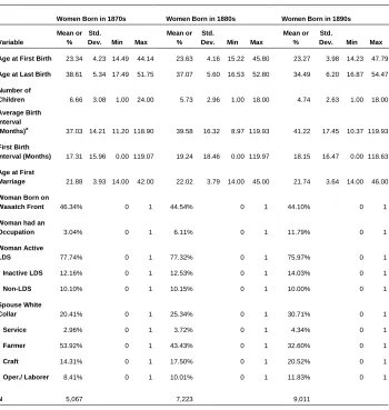
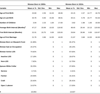
spouse‟s occupation is unknown, unreported, or insufficiently detailed to classify, and a very small number of cases in which spouses were reported to be in the military. Table 1 indicates the number of women in each ten-year birth cohort in our data set, increasing from 1,470 in the 1850s cohort to over 13,000 in the 1910s cohort.

Table 1: Means for regression data set and each birth cohort

All Cohorts Women Born in 1850s Women Born in 1860s

Variable

Mean or %

Std.

Dev. Min Max

Mean or %

Std.

Dev. Min Max

Mean or %

Std.

Dev. Min Max

Age at First Birth 23.48 4.29 14.23 54.93 20.91 3.30 15.02 43.54 22.08 3.92 14.65 54.93

Age at Last Birth 35.60 6.23 15.06 54.93 40.34 4.78 16.64 53.93 39.60 4.89 18.86 54.93

Number of

Children 5.02 2.91 1.00 24.00 8.95 3.04 1.00 20.00 7.82 3.05 1.00 17.00

Average Birth

Interval (Months)a

42.79 18.69 8.97 119.93 32.28 10.22 18.40 117.75 34.53 11.98 13.23 118.73

First Birth

Interval (Months) 21.90 21.16 0.00 120.00 15.86 11.83 0.90 115.87 16.16 13.25 0.00 112.87

Age at Marriage 21.65 3.79 14.00 53.00 19.60 3.17 14.00 42.00 20.72 3.76 14.00 53.00

Woman Born on

Wasatch Front 45.87% 0 1 78.03% 0 1 52.28% 0 1

Woman had an

Occupation 16.39% 0 1 3.88% 0 1 3.31% 0 1

Woman Active

LDS 74.25% 0 1 81.36% 0 1 78.31% 0 1

Inactive LDS 15.24% 0 1 6.53% 0 1 9.98% 0 1

Non-LDS 10.50% 0 1 12.11% 0 1 11.71% 0 1

Spouse White

Collar 29.81% 0 1 14.29% 0 1 16.89% 0 1

Service 3.96% 0 1 1.43% 0 1 2.43% 0 1

Farmer 33.26% 0 1 66.87% 0 1 62.06% 0 1

Craft 20.51% 0 1 12.18% 0 1 12.38% 0 1

Oper./ Laborer 12.46% 0 1 5.24% 0 1 6.24% 0 1

N 49,728 1,470 4,847

a

(12)

Table 1: (Continued)

Women Born in 1870s Women Born in 1880s Women Born in 1890s

Variable

Mean or %

Std.

Dev. Min Max

Mean or %

Std.

Dev. Min Max

Mean or %

Std.

Dev. Min Max

Age at First Birth 23.34 4.23 14.49 44.14 23.63 4.16 15.22 45.80 23.27 3.98 14.23 47.79

Age at Last Birth 38.61 5.34 17.49 51.75 37.07 5.60 16.53 52.80 34.49 6.20 16.87 54.47

Number of

Children 6.66 3.08 1.00 24.00 5.73 2.96 1.00 18.00 4.74 2.63 1.00 18.00

Average Birth Interval

(Months)a 37.03 14.21 11.20 118.90 39.58 16.32 8.97 119.93 41.22 17.45 10.37 119.93

First Birth

Interval (Months) 17.31 15.96 0.00 119.07 19.24 18.46 0.00 119.97 18.15 16.47 0.00 118.63

Age at First

Marriage 21.88 3.93 14.00 42.00 22.02 3.79 14.00 45.00 21.74 3.64 14.00 46.00

Woman Born on

Wasatch Front 46.34% 0 1 44.54% 0 1 44.10% 0 1

Woman had an

Occupation 3.04% 0 1 6.11% 0 1 11.79% 0 1

Woman Active

LDS 77.74% 0 1 77.32% 0 1 75.97% 0 1

Inactive LDS 12.16% 0 1 12.53% 0 1 14.03% 0 1

Non-LDS 10.10% 0 1 10.15% 0 1 10.00% 0 1

Spouse White

Collar 20.41% 0 1 25.34% 0 1 30.71% 0 1

Service 2.96% 0 1 3.72% 0 1 4.34% 0 1

Farmer 53.92% 0 1 43.43% 0 1 32.60% 0 1

Craft 14.31% 0 1 17.50% 0 1 20.52% 0 1

Oper./ Laborer 8.41% 0 1 10.01% 0 1 11.83% 0 1

N 5,067 7,223 9,011

a

(13)

Women Born in 1900s Women Born in 1910s

Variable Mean or % Std. Dev. Min Max Mean or % Std. Dev. Min Max

Age at First Birth 23.60 4.56 14.43 46.66 24.15 4.37 14.77 44.76

Age at Last Birth 33.76 6.50 15.06 48.91 34.21 5.78 15.77 53.33

Number of Children 3.94 2.23 1.00 17.00 3.82 1.98 1.00 16.00

Average Birth Interval (Months)a

47.27 20.69 10.03 119.92 48.45 20.44 10.13 119.93

First Birth Interval (Months) 22.01 20.75 0.00 120.00 29.84 26.96 0.00 119.97

Age at First Marriage 21.76 3.96 14.00 44.00 21.67 3.68 14.00 44.00

Woman Born on Wasatch Front 41.96% 0 1 45.37% 0 1

Woman had an Occupation 24.37% 0 1 29.14% 0 1

Woman Active LDS 74.92% 0 1 67.63% 0 1

Inactive LDS 17.16% 0 1 19.67% 0 1

Non-LDS 7.92% 0 1 12.70% 0 1

Spouse White Collar 33.25% 0 1 37.83% 0 1

Service 4.71% 0 1 4.31% 0 1

Farmer 24.55% 0 1 15.41% 0 1

Craft 23.42% 0 1 25.41% 0 1

Oper./ Laborer 14.07% 0 1 17.03% 0 1

N 10,064 13,027

a

The calculation of inter-birth interval includes only those who had at least two births. The overall N for this group is 45,266. For each cohort, the N’s are 1,453 in the 1850s, 3,343 in the 1860s, 6,827 in the 1870s, 6,827 in the 1880s, 8,266 in the 1890s, 8,839 in the 1900s, and 11,691 in the 1910s.

(14)

supervisors, carpenters, mining machine operators, and production supervisors), and operatives and laborers (including truck drivers, locomotive operating occupations, and undifferentiated laborers).7 Our observations begin with women born in 1850, soon after the Mormon pioneers entered the Utah territory, and the occupational distribution reflects the importance of agriculture in these early years: About two-thirds of the women in our 1850s birth cohort were married to farmers (see Table 1). Yet by the 1880s birth cohort, the share of these women who were married to farmers had fallen below half, and the farming share was only 15 percent among the husbands of the 1910s birth cohort. White collar occupations and both craft and operative/laborer blue collar positions grew substantially in importance in these years.

This scheme provides a rough SES ranking but also highlights other occupation-related factors that may affect the timing of family formation and fertility levels. Farm families typically “produced their own work force,” which promoted higher levels of fertility, while white collar work might require longer periods of schooling or training, which could delay family formation. Periods of training for craft workers could have a similar impact. As we noted above, this categorization might also map into differences in education and exposure to new ideas, although we do not have access to independent information on literacy or education level in these data.

In addition to the woman‟s birth cohort and her spouse‟s occupation, we control for several other factors that were correlated with family size in Utah in this era. One obvious factor of importance is religious background. Information on religious affiliation is fairly rare in historical records in the US, such as the Census. Hacker (1999) deals with this problem creatively by comparing the fertility of women who gave their children “biblical”‟ names to that of women who did not use such names. He finds higher levels of fertility among the former. Our records have more direct information on the strength of affiliation of women with the dominant religious group in Utah, the LDS Church. The UPDB contains information on baptism and endowment dates from family history records, and this was used to classify individuals as active members of the church, inactive members, or non-members. Individuals were

7_{For white collar workers, we use Census 1990 occupation codes 3 to 391. For service work, we use 403 to}

(15)

considered active church members if endowed before age 40.8 Individuals with a baptism but no endowment date were considered inactive. Those with no recorded baptism were considered non-LDS. (We do not have information on the religious identity of the non-LDS.) Active LDS women make up about three-fourths of our sample through the 1900s cohort before falling to about 67 percent of the 1910s cohort. The inactive LDS group grew fairly steadily in importance, rising to nearly one fifth of the sample in the 1910s cohort. The non-LDS group grew primarily in the last cohort.

Bean, Mineau, and Anderton demonstrate the importance of geographic fertility differentials within Utah, so we also control for the woman‟s birth along the more densely populated Wasatch Front (Utah, Salt Lake, Weber, and Davis counties). The Wasatch Front share declined from 78 percent for the 1850s birth cohort to 46 percent among those born in the 1870s and changed little thereafter. Finally, we control for whether the woman had an occupation recorded on her death certificate. The number of women for whom an occupation was reported was less than four percent of the sample through the 1870s cohort but then rose rapidly to 29 percent among the 1910s cohort. Most commonly, these women were elementary school teachers, sales workers, secretaries, nurses, and cooks. This measure of occupation, like that used for these women‟s spouses, comes from death certificates. It is therefore not a clean measure of labor force participation or employment at any particular point in time and can not be easily compared to the kinds of point-in-time measures available in most other sources. Still, it is worth noting that the increase in reported occupation for the women in our dataset matches closely with the increase in labor force participation found by Goldin (1983) in her examination of Census data. Goldin reports labor force participation rates of less than five percent for married white women born between 1866 and 1875. This figure then ranges from about 15 percent (at age 20) to a peak of nearly 40 percent (at age 50) for married white women born between 1906 and 1915 (Goldin 1983: 713). Very few of the mothers in our data set have farming occupations reported on their death certificates, although we expect that many of them were engaged in the various economic activities related to life on a farm. We therefore expect that our measure acts as an indicator of labor market activity outside the home. Farming work and other kinds of home production are quite often missed in the Census and other sources of evidence on women‟s labor force participation in this period (Sobek 2006: 2-37).

Before examining fertility behavior by occupational status, we present differences in children ever born along the dimensions discussed above: the woman‟s LDS status, her birth place, and her occupation (see Table 2). In general, religious affiliation is correlated with fertility as we would expect, with active LDS women having just over

8_{An endowment ceremony is a formal ceremony recognizing a high level of commitment to living in}

(16)

one more child than non-LDS women on average, and with inactive LDS women having fertility levels between these two extremes. While all of these groups experienced substantial declines in fertility between the 1850s cohort and the 1910s cohort, the gap between active LDS women and non-LDS women did not change dramatically over time (so this stable gap in number of children came to constitute a larger percentage difference as the total number of children declined for all groups). The fertility gaps between women with a reported occupation and those without, and between Wasatch Front residents and others, were not as large as the differences by religious affiliation. These gaps tended to grow in the early years of fertility decline and then become smaller as childbearing converged somewhat across groups at a new, lower level in the 1910s cohort.

Table 2: Children ever born by mother’s birth cohort, employment, LDS

status, and birthplace

Mother’s Birth Cohort

1850s 1860s 1870s 1880s 1890s 1900s 1910s

Mother’s Employment

No Occupation 8.96 7.82 6.68 5.80 4.84 4.11 3.97

Some Occupation 8.76 7.55 5.81 4.65 3.99 3.41 3.46

Gap by Mother’s

Employment 0.20 0.28 0.88 1.15 0.85 0.70 0.51

Mother’s LDS Status

NonLDS 7.99 6.94 5.42 4.68 3.53 2.87 2.91

Inactive LDS 8.45 7.01 6.05 5.10 4.28 3.47 3.30

Active LDS 9.14 8.05 6.92 5.98 4.99 4.16 4.14

Gap by LDS Status 1.14 1.11 1.49 1.29 1.46 1.29 1.23

Mother’s Birthplace

Not born on Wasatch Front 8.92 8.08 6.95 6.04 5.02 4.08 3.88

Born on Wasatch Front 8.96 7.58 6.32 5.35 4.40 3.75 3.75

Gap by Wasatch Front Birth -0.04 0.50 0.63 0.70 0.62 0.33 0.13

N 1470 3416 5067 7223 9011 10064 13027

(17)

Our primary interest, however, is fertility differences across spouse‟s occupation. Figures 1 through 5 present measures of several fertility-related behaviors grouped by the spouse‟s occupation and the woman‟s birth cohort. White collar families and farm families generally define the bounds of these behaviors. The “leadership” of white collar workers in terms of increase in age at marriage is apparent in Figure 1. After 1870, age at marriage stopped increasing. However, first birth interval (the time in months between marriage and first birth) rose considerably for all occupation groups for cohorts born after the 1890s (Figure 2), so that delay in the start of childbearing was driven by this mechanism in the latter part of our period.9

Figure 1: Age at marriage by mother's birth cohort and father's occupation

category

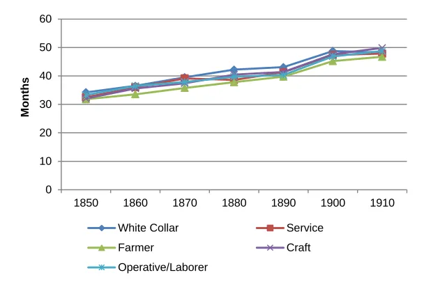
While the increase in first birth interval is concentrated after the 1890s, the average inter-birth interval (the average interval in months between each birth after the first) grew more gradually over time, with more modest acceleration after the 1890s (see Figure 3). The white collar – farmer gap in the length of the average inter-birth interval

9_{Ewbank (1991) emphasizes the role of lengthening birth intervals as a source of declining fertility in the}

mountain states, including Utah.

15 16 17 18 19 20 21 22 23 24

1850s 1860s 1870s 1880s 1890s 1900s 1910s

White Collar Service Farmer

(18)

rose over the first four cohorts, from about two months in the 1850 cohort to just over four months in the 1880s cohort, before declining back to its initial level.

While white collar families are distinctive in terms of age at marriage, farm families are the outliers when we measure age at last birth (Figure 4). As the stopping age declined substantially for all categories, the gap between farmers and white collar workers grew by over two years through the 1890s birth cohort, and all other occupational groups were clustered close to white collar workers. The age at last birth then rose somewhat for white collar workers over the last two cohorts, approaching the stopping age for farm families by that point. Finally, the number of children ever born declined steadily for all occupation groups across birth cohorts from the 1850s through the first decade of the 20th century before flattening out (see Figure 5). As with most of these measures, the gap between the white collar families and farm families rose for several decades and then declined, concentrating around a new fertility level at about half the initial value.

Figure 2: First birth interval by mother's birth cohort and father's occupation

0 5 10 15 20 25 30 35

1850 1860 1870 1880 1890 1900 1910

M

onths

White Collar Service

Farmer Craft

(19)

Figure 3: Average inter-birth interval by mother's birth cohort and father's occupation

To examine cross-occupational differences in the level and timing of change in these behaviors more formally, we estimate a series of regressions identifying the correlates of age at marriage, first birth interval, average inter-birth interval, age at last birth, and children ever born, incorporating dummy variables for spouse‟s occupational category and the woman‟s birth cohort along with interactions of occupation and cohort. We control for the woman‟s religious affiliation, place of birth (on the Wasatch Front or elsewhere in Utah), and whether or not she had a reported occupation. We also control for age at marriage in the analysis of birth intervals, age at last birth, and children ever born.

0 10 20 30 40 50 60

1850 1860 1870 1880 1890 1900 1910

M

ont

hs

White Collar Service

Farmer Craft

(20)

Figure 4: Age at last birth by mother's birth cohort and father's occupation category

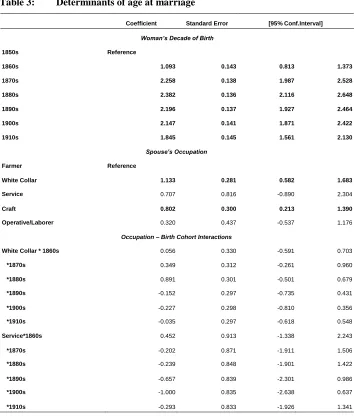
Results for age at marriage are found in Table 3. The main cohort effects indicate a general rise in age at marriage across cohorts from the 1850s to the 1860s and from the 1860s to the 1870s. There is then no further increase; in fact there is some decrease in age at marriage between the 1880s and 1890s cohorts and between the 1900s and 1910s cohorts (all of these differences are statistically significant in pairwise tests using a p value of .05). Women married to white collar and craft workers have somewhat higher marriage ages (compared to wives of farmers) in the main effects. The farmer/craft worker gap in marriage ages then declined after 1890.

30 32 34 36 38 40 42

1850s 1860s 1870s 1880s 1890s 1900s 1910s

(21)

Figure 5: Children ever born by mother's birth cohort and father's occupation category

0 1 2 3 4 5 6 7 8 9 10

1850s 1860s 1870s 1880s 1890s 1900s 1910s

(22)

Table 3: Determinants of age at marriage

Coefficient Standard Error [95% Conf.Interval]

Woman’s Decade of Birth

1850s Reference

1860s 1.093 0.143 0.813 1.373

1870s 2.258 0.138 1.987 2.528

1880s 2.382 0.136 2.116 2.648

1890s 2.196 0.137 1.927 2.464

1900s 2.147 0.141 1.871 2.422

1910s 1.845 0.145 1.561 2.130

Spouse’s Occupation

Farmer Reference

White Collar 1.133 0.281 0.582 1.683

Service 0.707 0.816 -0.890 2.304

Craft 0.802 0.300 0.213 1.390

Operative/Laborer 0.320 0.437 -0.537 1.176

Occupation – Birth Cohort Interactions

White Collar * 1860s 0.056 0.330 -0.591 0.703

*1870s 0.349 0.312 -0.261 0.960

*1880s 0.891 0.301 -0.501 0.679

*1890s -0.152 0.297 -0.735 0.431

*1900s -0.227 0.298 -0.810 0.356

*1910s -0.035 0.297 -0.618 0.548

Service*1860s 0.452 0.913 -1.338 2.243

*1870s -0.202 0.871 -1.911 1.506

*1880s -0.239 0.848 -1.901 1.422

*1890s -0.657 0.839 -2.301 0.986

*1900s -1.000 0.835 -2.638 0.637

*1910s -0.293 0.833 -1.926 1.341

Adj R2

(23)

Craft*1860s 0.110 0.359 -0.593 0.814

*1870s -0.194 0.338 -0.856 0.467

*1880s -0.446 0.324 -1.081 0.190

*1890s -0.824 0.320 -1.450 -0.197

*1900s -0.998 0.318 -1.623 -0.374

*1910s -0.970 0.318 -1.593 -0.346

Op/Lab*1860s 0.826 0.511 -0.177 1.828

*1870s 0.023 0.478 -0.913 0.959

*1880s -0.014 0.463 -0.921 0.893

*1890s -0.561 0.457 -1.456 0.334

*1900s -0.561 0.454 -1.451 0.329

*1910s -0.429 0.452 -1.314 0.456

Woman’s LDS Status

Non-LDS Reference

ActiveLDS 0.269 0.055 0.161 0.378

InActiveLDS -0.041 0.067 -0.173 0.090

Woman born on Wasatch Front 0.366 0.034 0.299 0.433

Occupation Reported for Woman 1.127 0.048 1.034 1.221

Constant 18.788 0.130 18.533 19.043

Adj R2

= .052, N=49,278 / Bold => p value < .05

Similar results for first birth interval are reported in Table 4. There is a statistically significant increase in first birth interval between the 1870s and 1880s cohort (p value = .01) but then some retrogression in this increase in the 1890s. Increases then re-appear between the 1890s and 1900s (p value = .001) and 1900s and 1910s (p value = .000) cohorts. There are no initial differences across occupations in the main effects, but white collar families are characterized by greater increases in first birth intervals, compared to farmers, by the 1900s.10

10_{We incorporate all first births in these calculations, including those likely to have arisen from pre-marital}

(24)

Table 4: Determinants of first birth interval

1860s -0.279 0.781 -1.810 1.252

1870s -0.013 0.756 -1.495 1.469

1880s 1.311 0.744 -0.148 2.770

1890s 0.741 0.750 -0.730 2.122

1900s 2.664 0.770 1.155 4.173

1910s 8.410 0.795 6.853 9.968

White Collar 1.263 1.535 -1.745 4.271

Service -0.538 4.451 -9.263 8.186

Craft 0.180 1.640 -3.035 3.395

Operative/Laborer -0.232 2.388 -4.914 4.449

White Collar * 1860s -0.098 1.803 -3.633 3.437

*1870s 1.841 1.702 -1.496 5.177

*1880s 2.194 1.645 -1.031 5.419

*1890s 0.613 1.625 -2.572 3.798

*1900s 4.487 1.626 1.301 7.674

*1910s 5.461 1.625 2.275 8.646

Adj. R2=.091 N=49,278 / Bold => p value < .05

(25)

Service*1860s 3.632 4.991 -6.151 13.415

*1870s 1.081 4.762 -8.253 10.414

*1880s 0.745 4.632 -8.334 9.824

*1890s 1.931 4.581 -7.050 10.912

*1900s 0.090 4.565 -8.857 9.038

*1910s 3.957 4.554 -4.969 12.884

Craft*1860s 0.136 1.961 -3.708 3.979

*1870s 0.611 1.844 -3.004 4.226

*1880s 1.320 1.773 -2.154 4.795

*1890s 0.151 1.746 -3.272 3.575

*1900s 1.648 1.741 -1.763 5.055

*1910s 3.259 1.737 -0.147 6.664

Op/Lab*1860s 0.728 2.795 -4.749 6.206

*1870s 1.218 2.610 -3.897 6.333

*1880s 1.888 2.530 -3.070 6.846

*1890s 0.597 2.495 -4.294 5.487

*1900s 1.454 2.482 -3.410 6.318

*1910s 2.683 2.468 -2.155 7.521

ActiveLDS -8.732 0.301 -9.322 -8.141

InActiveLDS -5.313 0.366 -6.030 -4.595

Age at Marriage 0.401 0.025 0.352 0.449

Occupation Reported for Woman 2.183 0.263 1.669 2.698

Constant 23.572 0.715 22.170 24.974

(26)

The pattern of change for average inter-birth intervals is somewhat different (see Table 5). Here, an increase in the main cohort effects is present from the 1860s on, with intervals increasing monotonically and statistically significantly across cohorts (with p values below .05 in pairwise comparisons) through the 1910s. White collar families always have longer average birth intervals than do farm families (as is evident in the main occupation effects), but there are no statistically significant occupation*cohort interaction effects.

Table 5: Determinants of average inter-birth interval

1860s 2.338 0.694 0.977 3.697

1870s 5.155 0.673 3.837 6.473

1880s 7.259 0.663 5.960 8.558

1890s 9.172 0.670 7.860 10.485

1900s 14.676 0.692 13.320 16.033

1910s 15.984 0.713 14.586 17.382

White Collar 2.855 1.364 0.181 5.529

Service 0.459 3.931 -7.246 8.163

Craft 0.471 1.460 -2.390 3.332

Operative/Laborer 1.429 2.136 -2.757 5.615

White Collar * 1860s 0.433 1.608 -2.718 3.585

*1870s 1.367 1.521 -1.614 4.348

*1880s 1.987 1.467 -0.889 4.863

*1890s 0.737 1.451 -2.106 3.581

*1900s 1.051 1.454 -1.799 3.900

*1910s -1.041 1.451 -3.885 1.802

Service*1860s 1.900 4.448 -6.817 10.618

*1870s 2.816 4.220 -5.454 11.087

Adj. R2

(27)

*1880s 0.212 4.103 -7.830 8.254

*1890s 1.023 4.058 -6.932 8.977

*1900s 1.311 4.047 -6.620 9.243

*1910s 0.643 4.034 -7.263 8.549

Craft*1860s 1.708 1.747 -1.717 5.132

*1870s 1.138 1.647 -2.090 4.365

*1880s 2.023 1.582 -1.078 5.125

*1890s 0.844 1.560 -2.213 3.901

*1900s 1.591 1.558 -1.462 4.644

*1910s 2.214 1.553 -0.830 5.257

Op/Lab*1860s 1.563 2.495 -3.328 6.453

*1870s 0.339 2.342 -4.251 4.929

*1880s 0.209 2.268 -4.236 4.654

*1890s -1.386 2.236 -5.769 2.997

*1900s -0.235 2.227 -4.600 4.130

*1910s 0.100 2.212 -4.236 4.435

ActiveLDS -3.104 0.292 -3.676 -2.532

InActiveLDS -1.431 0.354 -2.124 -0.738

Age at Marriage -0.446 0.024 -0.493 -0.398

Occupation Reported for Woman -0.054 0.247 -0.539 0.430

Constant 33.028 0.645 31.764 34.292

Adj. R2

=.090 N=45,266 / Bold => p value < .05

(28)

collar families exceeds that of farm families by the 1870s cohort, and this statistical difference persists through the 1890s cohort. Both groups of blue collar workers (craft and operative/laborer) experienced greater declines in age at last birth than did farm families in both the 1880s and 1890s birth cohorts. The differential pace of decline in age at last birth for service workers‟ families, compared to farm families, is of a similar magnitude. However, the number of service workers is fairly small, and none of their interaction effects are statistically significant at conventional levels. There are no differences across any other occupation pairings in the interaction effects.11

Table 6: Determinants of age at last birth

1860s -0.969 0.215 -1.390 -0.548

1870s -1.950 0.208 -2.357 -1.543

1880s -3.170 0.204 -3.571 -2.769

1890s -5.230 0.206 -5.634 -4.826

1900s -6.319 0.211 -6.733 -5.904

1910s -6.195 0.218 -6.623 -5.767

White Collar -0.695 0.421 -1.521 0.132

Service -0.856 1.223 -3.252 1.540

Craft -0.635 0.451 -1.518 0.248

White Collar * 1860s -0.504 0.495 -1.475 0.467

*1870s -1.579 0.468 -2.495 -0.662

*1880s -1.761 0.452 -2.647 -0.875

Adj. R2

=.090 N=45,266 / Bold => p value < .05

11_{In Dribe et al (2013), we examine risk of first birth and risk of higher order birth in a proportional hazards}

(29)

*1890s -1.952 0.446 -2.827 -1.077

*1900s -0.658 0.447 -1.534 0.217

*1910s 0.444 0.446 -0.431 1.319

Service*1860s -0.495 1.371 -3.182 2.192

*1870s -1.592 1.308 -4.156 0.971

*1880s -1.198 1.272 -3.692 1.295

*1890s -1.699 1.258 -4.165 0.768

*1900s -1.066 1.254 -3.524 1.391

*1910s -0.249 1.251 -2.701 2.202

Craft*1860s -0.169 0.539 -1.225 0.887

*1870s -0.682 0.507 -1.674 0.311

*1880s -1.186 0.487 -2.141 -0.232

*1890s -1.359 0.480 -2.299 -0.419

*1900s -0.771 0.478 -1.708 0.166

*1910s -0.208 0.477 -1.143 0.727

Op/Lab*1860s -0.632 0.768 -2.137 0.872

*1870s -1.141 0.717 -2.546 0.264

*1880s -1.426 0.695 -2.788 -0.065

*1890s -1.391 0.685 -2.734 -0.048

*1900s -1.042 0.682 -2.377 0.294

*1910s -0.352 0.678 -1.680 0.977

ActiveLDS 2.591 0.083 2.429 2.753

InActiveLDS 0.578 0.101 0.381 0.775

Woman born on Wasatch Front -0.259 0.051 -0.359 -0.158

Age at Marriage 0.370 0.007 0.357 0.383

Occupation Reported for Woman -0.902 0.072 -1.044 -0.761

Constant 39.379 0.196 30.995 39.764

Adj R2 = .209, N=49,278 / Bold => p value < .05

(30)

Table 7).12 White collar families begin with a lower level of childbearing than is found among farm families, and they also experienced larger reductions from the 1870s through the 1900s. Service workers‟ families had greater reductions in childbearing than did farm families in both the 1890s and 1900s birth cohorts, craft workers‟ families had greater reductions from the 1870s on, and operative and laborers‟ families had greater reductions from the 1880s through the 1900s cohorts. White collar families had greater decreases in childbearing than did operative/laborer families in the 1890s cohort, although craft workers‟ families had greater reductions than did white collar families in the 1910s cohort.

Table 7: Determinants of children ever born

1860s -0.075 0.013 -0.101 -0.050

1870s -0.159 0.013 -0.185 -0.134

1880s -0.255 0.013 -0.280 -0.230

1890s -0.422 0.013 -0.448 -0.396

1900s -0.603 0.014 -0.631 -0.575

1910s -0.650 0.015 -0.680 -0.620

White Collar -0.076 0.026 -0.127 -0.024

Service -0.019 0.076 -0.168 0.130

Craft -0.011 0.027 -0.065 0.042

White Collar * 1860s -0.025 0.032 -0.087 0.037

*1870s -0.112 0.030 -0.172 -0.053

*1880s -0.176 0.029 -0.233 -0.118

*1890s -0.191 0.029 -0.248 -0.134

Generalized Linear Model, Poisson distribution. N=49,278 / Bold => p value < .05

(31)

*1900s _-0.135 _0.030 _-0.193 _-0.077

*1910s

-0.019 0.029 -0.076 0.039

Service*1860s _-0.127 _0.087 _-0.298 _0.045

*1870s _-0.156 _0.083 _-0.320 _0.007

*1880s

-0.120 0.081 -0.278 0.037

*1890s

-0.200 0.080 -0.357 -0.043

*1900s _-0.163 _0.080 _-0.320 _-0.006

*1910s

-0.123 0.080 -0.279 0.034

Craft*1860s

-0.049 0.034 -0.115 0.017

*1870s _-0.071 _0.032 _-0.134 _-0.009

*1880s _-0.144 _0.031 _-0.205 _-0.084

*1890s

-0.144 0.030 -0.204 -0.085

*1900s

-0.130 0.031 -0.190 -0.070

*1910s _-0.114 _0.031 _-0.174 _-0.054

Op/Lab*1860s

-0.052 0.048 -0.147 0.043

*1870s

-0.067 0.045 -0.156 0.021

*1880s _-0.111 _0.044 _-0.197 _-0.026

*1890s

-0.086 0.043 -0.170 -0.001

*1900s

-0.095 0.043 -0.180 -0.011

*1910s _-0.064 _0.043 _-0.148 _0.020

ActiveLDS 0.277 0.007 0.263 0.292

InActiveLDS 0.096 0.009 0.078 0.114

Woman born on Wasatch Front -0.032 0.004 -0.040 -0.024

Age at Marriage -0.045 0.001 -0.046 -0.044

Occupation Reported for Woman -0.095 0.007 -0.108 -0.082

Constant 1.895 0.013 1.870 1.921

(32)

Our control variables generally have statistically significant and right-signed coefficients.13 It might seem surprising that active LDS women had a later age at marriage than did non-LDS women, but this is consistent with Bean et al.‟s findings for the late 1800s (Bean et al. 1990: 169). The one other surprise is in the lack of significant effect of the woman‟s own employment on average inter-birth interval. It may be that the occupation reported on these women‟s death certificates reflects employment before childbearing, as it affects age at marriage and first birth interval. It might also reflect employment after a desired family size is reached, as woman‟s own employment reduced both children ever born and age at last birth. During their childbearing years, however, these women may have remained out of the labor market, so that inter-birth intervals were not substantially affected by employment.

To summarize the patterns of correlation of fertility behavior with spouse‟s occupation, we find that delays in the beginning of family formation are driven by rising age at marriage initially and by longer first birth intervals in later cohorts. White collar families experienced larger increases in first birth interval than did farm families by the end of the period we examine. Average inter-birth intervals increased generally and steadily beginning in the 1860s cohort, and white collar families typically had longer intervals than did farm families, but there were no notable distinctions across occupations in the timing of change in these intervals. Age at last birth and the number of children ever born declined generally and continually. White collar families were “leaders” here to a degree, although most other categories of families also became distinct from farm families on these dimensions over time.

5. Conclusion and discussion

We have uncovered some intriguing interactions between socio-economic status (as measured by spouse‟s occupation) and fertility change in Utah in the era of the fertility transition. Even though all groups experienced considerable decline in fertility, the specific paths to this decline differed in ways that may be tied to economic imperatives. Families of white collar workers led many of these changes, particularly those relating to the starting of family life, perhaps reflecting the impact of longer periods of education or training and early career transitions. Farm families were particularly distinctive in the late ages at which they continued to add children and also in the number of children ever born, perhaps reflecting an ongoing need for family labor in agriculture, especially to support aging parents.

(33)

Interpreting these patterns of change requires attention to the economic context. For instance, agriculture‟s share of total employment declined considerably during the period we are studying. It is possible that the farmers in our earliest cohorts were engaged in a variety of activities beyond agriculture, while those who remained in farming at the end may have been substantially more specialized. These kinds of changes could affect the impact of father‟s occupation on fertility and in particular our ability to see cross-occupational differences.14

We have only begun to exploit the rich resources of the UPDB for studying fertility change. One area of extension could include looking at broader networks beyond the nuclear family. Might the socio-economic status of grandparents, and of parent‟s siblings, have had an influence on fertility behavior? While the frontier setting of our analysis, and the prominent role of a unique religious culture in this community, will require us to be cautious about the generalizability of our findings, we believe the opportunity to improve our understanding of fertility change and economic-demographic interaction through the resources of the UPDB is substantial.

6. Acknowledgements

This work was supported by in part by the National Institutes of Health grant AG022095 (The Utah Study of Fertility, Longevity and Aging). We wish to thank the Huntsman Cancer Foundation for database support provided to the Pedigree and Population Resource of the HCI, University of Utah. Partial support for all datasets within the UPDB was provided by the University of Utah HCI and the HCI Cancer Center Support Grant, P30 CA42014 from National Cancer Institute.

This paper was presented in a session on “Social Class and Fertility Before, During, and After the Fertility Transition” at the Social Science History Association meetings, Vancouver, British Columbia, November 2012. We are grateful for the comments and suggestions of participants in that session.

14_{As a first test of this hypothesis, we reran the analysis adding an interaction of “Woman Born on Wasatch}

(34)

References

Bean, L.L., Mineau, G.P., and Anderton, D.L. (1990). Fertility Change on the American Frontier: Adaptation and Innovation. Berkeley: University of California Press.

Carson, S.A. (2001). Indentured migration in America‟s great basin: an observation in strategic behavior in cooperative exchanges. Journal of Institutional and

Theoretical Economics 159(4): 651676. doi:10.1628/0932456012974440.

Carter, S.B., Ransom, R.L., and Sutch, R. (2004). Family matters: The life-cycle transition and the antebellum American fertility decline. In: Guinnane, T.W., Sundstrom, W.A., and Whatley, W.C. (eds.). History matters: Essays on economic growth, technology, and demographic change. Stanford: Stanford University Press: 271327.

David, P.A. and Sanderson, W.C. (1987). The emergence of a two-child norm among American birth-controllers. Population and Development Review 13(1): 141.

doi:10.2307/1972119.

David, P. and Sanderson, W. (1992). Rudimentary contraceptive methods and the American transition to marital fertility control, 1855-1915. In: Engerman, S.L. and Gallman, R.E. (eds.). Long Term Factors in American Economic Growth. Chicago: University of Chicago Press: 307379.

Dribe, M., Bras, H., Bresci, M., Gagnon, A., Gauvreau, D., Hanson, H., Maloney, T., Mazzoni, S., Molitoris, J., Pozzi, L., Smith, K.R., and Vézina, H. (2013). Socioeconomic status and fertility: Insights from historical transitions in Europe and North America. Washington, DC, Paper presented at the annual meetings of the Economic History Association.

Easterlin, R.A. (1976). Population change and farm settlement in the northern United States. Journal of Economic History 36(1): 4575. doi:10.1017/S0022050700 09450X.

Ewbank, D.C. (1991). The marital fertility of American whites before 1920. Historical

Methods 24(4): 141170. doi:10.1080/01615440.1991.9955301.

(35)

Goldin, C. (1983). The changing economic role of women: A quantitative approach. Journal of Interdisciplinary History 13(4): 707733. doi:10.2307/203887. Guest, A.M. (1981). Social structure and US inter-state fertility differentials in 1900.

Demography 18(4): 465486. doi:10.2307/2060943.

Guinnane, T.W., Moehling, C.M., and O‟Grada, C. (2006). The fertility of the Irish in the United States in 1910. Explorations in Economic History 43(3): 465485.

doi:10.1016/j.eeh.2005.04.002.

Guinnane, T.W. (2011). The historical fertility transition: A guide for economists. Journal of Economic Literature 49(3): 589614. doi:10.1257/jel.49.3.589. Hacker, J.D. (1999). Child naming, religion, and the decline of marital fertility in

nineteenth-century America. The History of the Family 4(3): 339365.

doi:10.1016/S1081-602X(99)00019-6.

Hacker, J.D. (2003). Rethinking the „early‟ decline of marital fertility in the United States. Demography 40(4): 605620. doi:10.2307/1515199.

Haines, M.R. (1978). Fertility decline in industrial America: An analysis of the Pennsylvania anthracite region, 1850-1900, using „own children‟ methods. Population Studies 32(2): 327354. doi:10.2307/2173565.

Haines, M.R. (1990). Western fertility in mid-transition: Fertility and nuptiality in the United States and selected nations at the turn of the century. Journal of Family History 15(1): 2348. doi:10.1177/036319909001500102.

Haines, M.R. (1992). Occupation and social class during fertility decline: Historical perspectives. In Gillis, J.R., Tilley, L.A., and Levine, D. (eds.). The European Experience of Declining Fertility, 1850-1970. Oxford: Oxford University Press: 193226.

Haines, M.R. (2000). The white population of the United States, 1790-1920. In: Haines, M.R. and Steckel, R.H. (eds.). A population history of North America. Cambridge: Cambridge University Press: 305369.

Haines, M.R. and Guest, A.M. (2008). Fertility in New York state in the pre-Civil War era. Demography 45(2): 345361. doi:10.1353/dem.0.0009.

(36)

Murray, J.E. and Lagger, B.A. (2001). Involuntary childlessness and voluntary fertility control during the fertility transition: Evidence from men who graduated from an American college. Population Studies 55(1): 2536. doi:10.1080/0032472 0127676.

Pope, C.L. (1989). Households on the American frontier: The distribution of income and wealth in Utah, 1850-1900. In Galenson, D.W. (ed.). Markets in history: Economic studies of the past. Cambridge: Cambridge University Press: 148189.

Smith, D.S. and Hindus, M.S. (1975) Premarital pregnancy in America 1640-1971: An overview and interpretation. The Journal of Interdisciplinary History 5(4): 537570. doi:10.2307/202859.

Smith, D.S. (1996). The number and quality of children: Education and marital fertility in early twentieth-century Iowa. Journal of Social History 30(2): 367392.

doi:10.1353/jsh/30.2.367.

Smith, K.R. (2012) Pedigree and population resource: Utah population database.

Huntsman Cancer Institute, University of Utah.

http://www.huntsmancancer.org/groups/ppr/

Sobek, M. (2006). Occupations. In: Carter, S.B., Gartner, S.S., Haines, M.R., Olmstead, A.L., Sutch, R., and Wright, G. (eds.). Historical statistics of the United States: Earliest times to the present. Cambridge: Cambridge University Press: 3540. Steckel, R.H. (1992). The fertility transition in the United States: Tests of alternative

hypotheses. In Goldin, C. and Rockoff, H. (eds.). Strategic factors in nineteenth-century American economic history. Chicago: University of Chicago Press: 351374.

Sundstrom, W.A. and David, P.A. (1988). Old age security motives, labor markets, and farm family fertility in antebellum America. Explorations in Economic History 25(2): 164197. doi:10.1016/0014-4983(88)90015-0.

US Department, of Health and Human Services (2012). Guidelines for Reporting Occupation and Industry on Death Certificates. Washington: US Department of Health and Human Services. http://www.cdc.gov/niosh/docs/2012-149/pdfs/2012-149.pdf.