DEMOGRAPHIC RESEARCH
VOLUME 31, ARTICLE 25, PAGES 757
−
778
PUBLISHED 2 OCTOBER 2014
http://www.demographic-research.org/Volumes/Vol31/25/ DOI: 10.4054/DemRes.2014.31.25
Research Article
Exploring the population implications of male
preference when the sex probabilities at birth can
be altered
Frank T. Denton
Byron G. Spencer
© 2014 Frank T. Denton & Byron G. Spencer.
This open-access work is published under the terms of the Creative Commons Attribution NonCommercial License 2.0 Germany, which permits use, reproduction & distribution in any medium for non-commercial purposes, provided the original author(s) and source are given credit.
2 Stopping rules 759
3 An artificial population 763
4 Properties and implications of the Q matrix 765
5 Population effects of the stopping rules 766
6 Interaction of the fertility rate and the sex ratio at birth 769
7 The trade-off between fertility and the sex ratio at birth 771
8 Alternative survival rates and the rate of growth 772
9 Summary and discussion 773
10 Acknowledgements 775
Exploring the population implications of male preference when the
sex probabilities at birth can be altered
Frank T. Denton1 Byron G. Spencer2
Abstract
OBJECTIVE
The paper explores the population effects of male preference stopping rules and of alternative combinations of fertility rates and male-biased birth sex ratios.
METHODS
The ‘laboratory’ is a closed, stable population with five age groups and a dynamic process represented by a compact Leslie matrix. The new element is sex-selective abortion. We consider nine stopping rules, one with no male preference, two with male preference but no abortion, and six with male preference and the availability of abortion to achieve a desired number of male births. We calculate the probability distribution over the number of births and number of male births for each rule and work out the effects at the population level if the rule is adopted by all women bearing children. We then assess the impact of alternative combinations of fertility rates and male-biased sex ratios on the population.
RESULTS
In the absence of sex-selective abortion, stopping rules generally have no effect on the male/female birth proportions in the population, although they can alter the fertility rate, age distribution, and rate of growth. When sex-selective abortion is introduced the effect on male/female proportions may be considerable, and other effects may also be quite different. The contribution of this paper is the quantification of effects that might have been predictable in general but which require model-based calculations to see how large they can be. As the paper shows, they can in fact be very large: a population in which sex-selective abortion is widely practised can look quite different from what it would otherwise be.
1. Introduction
The theoretical consequences of sex-preference stopping rules at the family level have been known for a long time – in particular, the lack of any effect on the overall proportions of male and female births when the probabilities for individual births are fixed and the same throughout the population (Goodman 1961; Keyfitz 1968; and others). However, there is an accumulation of evidence now to indicate the use of abortion to alter those probabilities in favour of male births in countries where male preference is common; see Bongaarts (2013) for a recent survey of evidence of male preference and the use of sex-selective abortion. Some countries of Eastern and Southern Asia have received particular attention in that regard (see, for example, Guilmato 2010; Jiang, Li, and Feldman 2011) and there is evidence of the use of abortion by emigrants from those countries who are resident elsewhere: Dubuc and Coleman (2007); Almond and Edlund (2008); Abrevaya (2009); Almond, Edlund, and Milligan (2013); Ray, Henry, and Urquia (2012). (While male preference has received most of the attention in the literature, including the present paper, female preference is certainly possible also; see Fuse 2013, for evidence of that from Japan.) Yamaguchi (1989) explored the effects of stopping rules on birth order and number of siblings in the absence of direct parental control over the sex probabilities. More recently, Yadava, Kumar, and Srivistava (2013) investigated the effects on the sex probabilities at birth of stopping rules when selective abortion is an option. The question on which we focus here is a ‘what if’ question: What if there were a change in birth probabilities at the individual family level: how would that translate into changes in the characteristics of the population?
This is an exploratory paper. We explore, in particular, the potential effects of male preference stopping rules on a stable population and, more generally, the implications of higher male/female ratios at birth. We begin by choosing a set of nine stopping rules, three with no abortion and six with, and derive the associated probability functions at the individual family level. We simulate the consequences of each rule for the population as a whole – in particular, its rate of growth and age and sex distributions, were the rule to be adopted throughout the population. We then move away from the idea of explicit stopping rules, specify nine alternative sex ratios at birth (assuming unspecified rules or mixtures of rules underlying them), couple the ratios with alternative fertility rates, and derive the stable population growth rates and sex distributions that would result.
simulations, and can be easily used to derive the resultant stable populations. We note and discuss the properties of the matrix as a prelude to its application in the simulations. To emphasize that our population is artificial we think of it as being the population of a mythical country called Alpha. The population of Alpha then provides a laboratory in which to explore the population implications of family preferences for male children.
2. Stopping rules
We consider the nine rules that a family might adopt. (The choice is somewhat arbitrary but provides a wide range of population outcomes for analysis.) One of the rules assumes no male preference. Two others reflect male preference but no effective way of altering the probabilities of a particular male or female birth. The remaining ones allow for the possibility of knowing the sex of a child at an early stage of pregnancy and using selective abortion to increase the probability that the next birth will be a male. In specifying the rules we abstract from miscarriages and stillbirths, and assume that in the absence of sex-selective abortion a fetus would proceed to a live birth. We abstract also from the possibility of multiple births: all births are singletons. We label the stopping rules S0, S1, …, S8.
The rules fall into four categories. They differ with regard to male preference, preferences for family size, whether abortion is permitted and, if so, whether its use is limited or unlimited. Rule S0 is in category 1: it assumes no male preference and serves as a reference rule with which to compare the effects of the subsequent rules. Rules S1 and S2 fall into the second category: they assume male preference but no abortion option; S1 has a maximum number of births of three, S2 a maximum of four. Rules S3 and S4 fall into the third category: they assume male preference with limited use of abortion and maximum numbers of births of three and four, respectively. Rules S5–S8, which make up the fourth category, assume male preference with unlimited use of abortion: they have maxima of three, four, five, and six births, in that order. The main distinguishing feature of this latter category is that unlimited abortion allows exact determination of the number of males. The precise definitions of the rules are as follows.
S0: There is no male preference: stop only when the number of children ever born is three.
S1: Stop when the first male child is born or when the total number of children ever born is three, whichever comes first.
S3: Stop when the first male child is born. If there have been two births and no males, check the sex of the next fetus and abort if female. Allow the third birth to take place only if a fetus is male or there have been three successive abortions of female fetuses. The third birth will then be either male (with high probability) or female, and the three births will include one or no males. S4: Stop when the second male child is born. If there have been three births and
one or no males, check the sex of the next fetus and abort if female. Allow the fourth birth to take place if the fetus is male or there have been three successive abortions of female fetuses. The fourth birth will then be either male (with high probability) or female, and the four births will include two, one, or no males.
S5: Permit no more than one female birth; abort additional female fetuses, with no limit on the number of abortions. Stop when there are two male births. S6: Permit no more than one female birth; abort additional female fetuses, with
no limit on the number of abortions. Stop when there are three male births. S7: Permit no more than two female births; abort additional female fetuses, with
no limit on the number of abortions. Stop when there are three male births. S8: Permit no more than two female births; abort additional female fetuses, with
no limit on the number of abortions. Stop when there are four male births.
The joint probability functions for number of births (n) and number of male births (m) for these stopping rules are as follows, with p the probability of a male birth (assumed independent of parity), q = 1 − p the probability of a female birth, and a the probability of an abortion, which is set equal to the probability of a female fetus (a=q, but there is no birth); it is assumed, in the absence of abortion, that any fetus would survive to become a live birth. We put abortion functions in square brackets and place them in the probability expressions in that form to indicate their position in the sequence of births.
Rule S0: pmq m
m n m n P − = 3
0( , ) (for n= ,3 m=0,1,2,3)
Rule S1: pmqn m
m n n m n P − − − = 1 ) , (
1 (for n= ,12,3, m=1)
3
q
Rule S2: pmqn m m n n m n P − − − = 1 ) , (
2 (for n=2,3,4, m=2)
3
4pq
= (for n=4, m=1)
4
q
= (for n=4, m=0)
Rule S3: pmqn m
m n n m n P − − − = 1 ) , (
3 (for n= ,12, m=1)
= q² [1+α+α²+α³] p (for n= ,3 m=1) = q² [α³] q (for n= ,3 m=0)
Rule S4: pmqn m
m n n m n P − − − = 1 ) , (
4 (for n=2,3, m=2)
= 4q³ [1+α+α²+α³] p (for n=4, m=1)
= 3pq² [1+α+α²+α³] p (for n=4, m=2) = q³ [α³] q (for n=4, m=0)
Note: Rules S5 to S8 allow an unlimited number of abortions of unwanted female fetuses, and hence (in our theoretical framework) a desired male birth with certainty. In what follows, we use the symbol
[ ]
1 to indicate such a male birth with probability 1, as distinguished from a natural birth with probability p.Rule S5: 2
5(n,m) p
P = (for n=2, m=2)
= q[1] [1] + pq[1] (for n= ,3 m=2)
Rule S6: 3
6(n,m) p
P = (for n= ,3 m=3)
= q[1] [1] [1] + pq[1] [1] + p²q[1] (for n=4, m=3)
Rule S7: 3
7(n,m) p
P = (for n= ,3 m=3)
3
3qp
= (for n=4, m=3)
= q² [1] [1] [1] + 2pq
2 [1] [1] + 3p²q²[1]
(for n=5, m=3)
Rule S8: P8(n,m) = p4 (for n=4, m=4)
4
4qp
= (for n=5, m=4)
The numerical values of these probabilities are provided in Table 1. Cells with no entries represent impossible combinations of n and m, under the specified stopping rules, and show how the rules restrict the numbers of births and the male/female combinations. Also shown in the table are E(n) and E(m) (the expected numbers of births and male births), the proportion r=E(m)/E(n), and the corresponding male/female odds ratio, m/f = E(m) / (E(n) − E(m)). The probabilities assume m/f = 1.05 for an individual birth in the absence of sex selection – a ratio common to many countries (U.S., U.K., Canada and others) – and that is also the overall ratio calculated from the expected values for stopping rules S0, S1, and S2. With a limited possibility of sex selection through abortion (maximum three times) the male/female ratio rises to 1.3 or 1.4 (stopping rules S3, S4). With unlimited use of the abortion option (rules S5 to S8) it goes as high as 3.5 (in rule S6). (The assumption of an unlimited number of abortions is a matter of theoretical convenience. A more realistic interpretation would be that the number of abortions is limited but with a maximum sufficient to drive the probability of a male birth close to 1.)
Table 1: Probability distributions and related statistics at the family level: numbers of births and numbers of male births under alternative stopping rules
Number of births (n)
Number of males (m)
Prob(n,m) under given stopping rule
S0 S1 S2 S3 S4 S5 S6 S7 S8
1 0 -- -- -- -- -- -- -- -- --
1 1 -- 0.512 -- 0.512 -- -- -- -- --
2 0 -- -- -- -- -- -- -- -- --
2 1 -- 0.250 -- 0.250 -- -- -- -- --
2 2 -- -- 0.262 -- 0.262 0.262 -- -- --
3 0 0.116 0.116 -- 0.013 -- -- -- -- --
3 1 0.366 0.122 -- 0.224 -- -- -- -- --
3 2 0.384 -- 0.256 -- 0.256 0.738 -- -- --
3 3 0.134 -- -- -- -- -- 0.134 0.134 --
4 0 -- -- 0.057 -- 0.007 -- -- -- --
4 1 -- -- 0.238 -- 0.130 -- -- -- --
4 2 -- -- 0.187 -- 0.345 -- -- -- --
4 3 -- -- -- -- -- -- 0.866 0.197 --
Table 1: (Continued)
Number of births (n)
Number of males (m)
Prob(n,m) under given stopping rule
S0 S1 S2 S3 S4 S5 S6 S7 S8
5 0 -- -- -- -- -- -- -- -- --
5 1 -- -- -- -- -- -- -- -- --
5 2 -- -- -- -- -- -- -- -- --
5 3 -- -- -- -- -- -- -- 0.669 --
5 4 -- -- -- -- -- -- -- -- 0.134
5 5 -- -- -- -- -- -- -- -- --
6 0 -- -- -- -- -- -- -- -- --
6 1 -- -- -- -- -- -- -- -- --
6 2 -- -- -- -- -- -- -- -- --
6 3 -- -- -- -- -- -- -- -- --
6 4 -- -- -- -- -- -- -- -- 0.797
E(n) 3.000 1.726 3.219 1.726 3.219 2.738 3.866 4.535 5.728
E(m) 1.537 0.884 1.649 0.987 1.857 2.000 3.000 3.000 4.000
E(m)/E(n) 0.512 0.512 0.512 0.572 0.577 0.731 0.776 0.662 0.698 m/f ratio 1.050 1.050 1.050 1.335 1.362 2.711 3.466 1.955 2.315
Note: In the absence of selective abortion a birth is assumed to be male with probability .5122. A double dash indicates an impossible n,m combination.
3. An artificial population
women in that group bear all the children. (This simplification is convenient since it avoids having to deal with the age distribution of fertility rates, which is of little relevance for present purposes.) The population of Alpha provides a laboratory in which to ask what the aggregate effects would be of childbearing decisions made at the individual family level.
The first five rows of the Q matrix are for females, the last five for males. The )
2 , 1 (
Q cell is calculated, for female babies, as sf0rfF, where F is the fertility rate for
Young Adult females (the total fertility rate, since there is only the one childbearing age group), rf is the proportion of females at birth, and sf0 is the survivor correction for female births (Kintner, 2008, p. 323). Correspondingly, for male babies, the Q(6,2) cell is calculated as sm0rmF. The values of rm, rf (=1−rm), and F are set experimentally, at various levels; sf0 and sm0 are parameters with fixed values.
The group-to-group survival rates are in the normal positions for a Leslie matrix:
sf1 to sf4 in cells Q(21,),Q(3,2),Q(4,3),Q(5,4) for females, sm1 to sm4 in cells
) 9 , 10 ( ), 8 , 9 ( ), 7 , 8 ( ), 6 , 7
( Q Q Q
Q for males. We draw on 2001 Canadian life tables for
calibration of the survival rates: the rates are derived from the Lx values in those tables. (The Canadian life tables are based on mortality data for the three years 2000, 2001, and 2002 but are commonly referred to as 2001 tables; see Statistics Canada 2006.) The matrix itself is presented in Table 2, with the survival rates shown in numerical form, as calibrated values, and the fertility elements (which vary from experiment to experiment) in symbolic form.
Table 2: The Q matrix for a stable Alpha population with calibrated survival
rates
Col. 1 Col. 2 Col. 3 Col. 4 Col. 5 Col. 6 Col. 7 Col. 8 Col. 9 Col. 10
Row 1 0 sf0rfF 0 0 0 0 0 0 0 0
Row 2 0.9942 0 0 0 0 0 0 0 0 0
Row 3 0 0.9769 0 0 0 0 0 0 0 0
Row 4 0 0 0.8635 0 0 0 0 0 0 0
Row 5 0 0 0 0.3798 0 0 0 0 0 0
Row 6 0 sm0rmF 0 0 0 0 0 0 0 0
Row 7 0 0 0 0 0 0.9875 0 0 0 0
Row 8 0 0 0 0 0 0 0.9617 0 0 0
Row 9 0 0 0 0 0 0 0 0.7850 0 0
Row 10 0 0 0 0 0 0 0 0 0.2575 0
Note: sf0 = .9940, sm0 = .9924.
Each age group in the Alpha population consists of 20 years; correspondingly, the time interval can be thought of as 20 years, and be referred to as a generation. Now let
0
X be a column vector representing the population at time 0. With Q fixed the population k generations later is given by Xk =QkX0. For an arbitrary initial specification of X0 the population can be converted to stable form by letting k increase until there is no further change in the proportionate age distribution. This provides a convenient procedure for simulating the effects of different specifications of
F and rf . (The Perron-Frobenius theorem, as adapted to a Leslie matrix, ensures full
ergodicity in the sense of nondegenerate convergence to a stable population with growth rate independent of the initial population vector, as long as the first two elements of the vector are not both zero. The age/sex structure of the stable population is also independent of the initial vector – in the sense discussed in the next section – for a sufficiently wide range of choices to make the process ergodic in that regard too, for practical purposes; any reasonable choice of an initial vector will do. See Cull and Vogt 1973; Cohen 1979; and Keyfitz and Caswell, 2005, chapter 7.)
4. Properties and implications of the Q matrix
The Q matrix has the following feature: the stable population form that it generates is cyclical. The matrix is imprimative, with index of imprimativity 2, and has exactly two real nonzero eigenvalues, equal in value but of opposite sign (Keyfitz and Caswell 2005). The cycle is two generations in length so that if stability is achieved the proportionate age distributions for Xk and Xk+2 are identical, and similarly for Xk+1 and Xk+3. Only if the stable population is also stationary does the cycle disappear, making both the sizes and the proportionate age distributions at k and k+1 the same (the nonzero eigenvalues are then 1 and -1). In the general case, to put it differently, the stable form of the population encompasses, in a 2-period sequence, both a birth effect and a subsequent echo effect resulting from the entry of last generation’s newborn children into the childbearing Young Adult group this generation. While the proportionate age distributions behave cyclically the average of every two consecutive age distributions is strictly stable and, following Cull and Vogt (1973), that is what we use in analysing stable population age distributions. The same is true of sex distributions.
have Xt+2=Q2Xt =(1+G)Xt and Xt+3=Q2Xt+1=(1+G)Xt+1, where G is the two-generation rate of growth. The average one-two-generation (20-year) growth rate is then
1 ) 1
( +G1/2− and the average annual rate is g=(1+G)1/40−1. As it is common to think of population growth in terms of annual rates we show the g values in reporting aggregate results below.
The link between the growth rate and the fertility rate and male/female ratio at birth can be established as follows. Let the elements of Xt be labeled Xti, i= ,1,10. Based on Xt+2 =Q2Xt =(1+G)Xt, the first element of Xt+2 (Children) is then
1 1
0 1 1 ,
2 f f f t (1 ) t
t s s r FX G X
X+ = = + , and hence g can be calculated as ( )1/40 1 0
1s r F −
sf f f .
Note that, for a given fertility rate and proportion of female births, the rate of growth depends entirely on the survival rates for female children: sf0, the survivor correction for female births, and sf1, the rate that determines the proportion of female children in one generation who survive to bear children in the next. All other survival rates are irrelevant for the growth rate. (That is a well-known result for a Leslie matrix; we note it here for use later in the paper.)
5. Population effects of the stopping rules
The effects of each of the nine family stopping rules on the stable population of Alpha are displayed in Table 3, assuming in each case that the rule is adopted throughout the population by all families that have children. The overall proportions of male births and the corresponding male/female ratios are shown at the top of the table, along with the fertility rates and annual population growth rates. It is assumed that the proportion of women who bear no children is 15% in Alpha, so that a fertility rate is calculated as .85 times the corresponding value in Table 1. (The choice of .85 for our fictitious country Alpha is arbitrary. For comparison, the proportion of women 40–44 in the United States who had given birth was reported as .82 for 2008 and .90 for 1976, based on data from the Current Survey of Population; see Livingston and Cohn 2010.) Otherwise it is assumed that all families adopt the same stopping rule. Also on display in the table are the age distributions of the population (averages over the stable two-period cycle) and the proportions of males in the five age groups.
The effects of a stopping rule on the population depend on the preferred number of male births incorporated into the rule as a goal, the ‘aggressiveness’ with which the goal is pursued (the total number of births permitted in pursuit of it), and whether or not an abortion option is available. Rule S0 has no male preference goal but simply an
overall fixed number of children, set at three. Rule S1 has a goal of one male birth, a willingness to allow up to three births to achieve that goal, and no abortion option. Rule S2 is similar but the goal is now two males, with up to four births permitted. As expected, the population sex ratio at birth is unaffected by the adoption of either S1 or S2: the male/female ratio at birth is 1.05 for each of the S0, S1, and S2 rules. (This result has been well known since the early work of Goodman 1961; Keyfitz 1968; and others.) However, the population fertility rate, growth rate, and age distribution can be very much affected by the choice of a rule, even if the sex ratio is not. S0, with its fixed three births per family, produces a population fertility rate of 2.550, well above the natural replacement rate (which is a little under 2.1), and a corresponding positive annual rate of growth of .517%. S1, with its stop-at-the-first-male restriction, lowers the fertility rate to 1.467 and induces a negative rate of growth, -.862% per annum. S2, on the other hand, has the opposite effect, pushing the fertility rate up to 2.736 and the growth rate well into the positive range, .695%. The sex ratio of the population is of course the same under each of the three rules but the age distribution varies greatly: in S1, 18.6% of the population are in the Children category, 9.4% in the Old category; in S3, 30.7% are Children, 4.5% are Old. Thus the introduction of a stopping rule that leaves the sex ratio at birth unchanged can have major effects on other characteristics of the population. This too is not a surprising result, but the calculations for rules S0, S1, and S2 in Table 3 provide some indication of the possible sizes of the effects for rules that have no abortion option.
The abortion option, the new element in the calculation of stable population effects, is introduced in stopping rules S3 to S8. The calculations in Table 3 for these rules indicate the possibilities for increasing the male/female ratio at birth by the use of this option, beyond the natural ratio of 1.05 that applied under the earlier rules. S3 and S4 impose a limit of three on the number of abortions allowed, S5 to S8 impose no limit.
Table 3: Stable Alpha populations resulting from alternative stopping rules
Stopping rule
S0 S1 S2 S3 S4 S5 S6 S7 S8
Proportion male births
(rm) 0.512 0.512 0.512 0.572 0.577 0.731 0.776 0.662 0.698
Male/female ratio at
birth 1.050 1.050 1.050 1.335 1.362 2.711 3.466 1.955 2.315
Fertility rate (F) 2.550 1.467 2.736 1.467 2.736 2.327 3.286 3.855 4.869 Annual % growth rate 0.517 -0.862 0.695 -1.184 0.339 -1.189 -0.793 0.637 0.936 Population age
distribution
– children 29.2 18.6 30.7 16.5 27.8 16.7 19.5 30.4 32.9
– young adults 26.1 21.9 26.5 20.8 25.8 21.1 22.6 26.5 27.1
– middle aged 22.8 25.3 22.3 25.5 23.3 25.8 25.6 22.6 21.7
– retired 17.0 24.8 16.0 26.6 17.8 26.5 24.1 16.2 14.6
– old 4.9 9.4 4.5 10.6 5.2 9.9 8.1 4.3 3.6
– all ages 100.0 100.0 100.0 100.0 100.0 100.0 100.0 100.0 100.0 Proportion males
– children 51.2 51.2 51.2 57.1 57.6 73.0 77.6 66.1 69.8
– young adults 51.0 51.0 51.0 57.0 57.5 72.9 77.5 66.0 69.7
– middle aged 50.6 50.6 50.6 56.6 57.1 72.6 77.2 65.6 69.3
– retired 48.2 48.2 48.2 54.2 54.7 70.6 75.5 63.4 67.3
– old 38.7 38.7 38.7 44.5 45.0 62.0 67.6 54.1 58.2
– all ages 49.9 49.1 50.0 54.9 56.3 71.2 76.1 65.0 68.9
Note: The proportion of women bearing no children is set at 15% for this table.
6. Interaction of the fertility rate and the sex ratio at birth
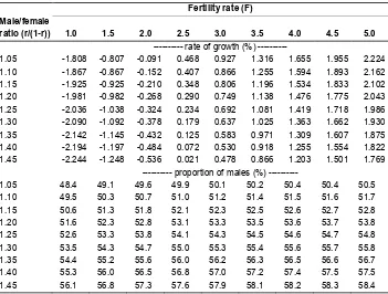
Now imagine that there is some unspecified set of stopping rules or mixture of stopping rules that prevails in the population of Alpha, with possible sex-selective abortion incorporated into the rules. Thus we move away from the idea of specifying particular rules and working out their implications, and simply consider alternative possible combinations of fertility rates and sex ratios at birth that might have resulted from such an unspecified set. (The ability to terminate pregnancies because of sex, coupled with possible heterogeneity of family choice of a rule across the population, would make virtually any such combination theoretically possible, over a range even wider than that which we now explore.) We focus in particular on the growth rate and the overall proportion of males in the stable population of our fictitious country Alpha, selecting nine alternative fertility rates, from 1.0 to 5.0, and coupling them with nine alternative male/female (m/ f) ratios, from 1.05 to 1.45. The results are presented in Table 4. The choice of fertility rates represents, in a rough way, a range of rates observed among countries in recent decades. The m/f ratios are a convenient choice for exploring the effects of variations in those ratios: the lower bound, 1.05, is a commonly observed ratio; the upper bound, 1.45, is an arbitrary value chosen for exploratory purposes – a very high value in comparison with ratios actually observed, although not as high as some of the hypothetical rule-generated ratios in Table 3.
Table 4: Annual rate of growth and proportion of males in a stable Alpha population with alternative combinations of fertility rates and male/female ratios at birth
Fertility rate (F) Male/female
ratio (r/(1-r)) 1.0 1.5 2.0 2.5 3.0 3.5 4.0 4.5 5.0
--- rate of growth (%) ---
1.05 -1.808 -0.807 -0.091 0.468 0.927 1.316 1.655 1.955 2.224
1.10 -1.867 -0.867 -0.152 0.407 0.866 1.255 1.594 1.893 2.162
1.15 -1.925 -0.925 -0.210 0.348 0.806 1.196 1.534 1.833 2.102
1.20 -1.981 -0.982 -0.268 0.290 0.749 1.138 1.476 1.775 2.043
1.25 -2.036 -1.038 -0.324 0.234 0.692 1.081 1.419 1.718 1.986
1.30 -2.090 -1.092 -0.378 0.179 0.637 1.025 1.363 1.662 1.930
1.35 -2.142 -1.145 -0.432 0.125 0.583 0.971 1.309 1.607 1.875
1.40 -2.194 -1.197 -0.484 0.072 0.530 0.918 1.255 1.554 1.822
1.45 -2.244 -1.248 -0.536 0.021 0.478 0.866 1.203 1.501 1.769
--- proportion of males (%) ---
1.05 48.4 49.1 49.6 49.9 50.1 50.2 50.4 50.4 50.5
1.10 49.5 50.3 50.7 51.0 51.2 51.4 51.5 51.6 51.7
1.15 50.6 51.3 51.8 52.1 52.3 52.5 52.6 52.7 52.8
1.20 51.6 52.3 52.8 53.1 53.3 53.5 53.6 53.7 53.8
1.25 52.6 53.3 53.8 54.1 54.3 54.5 54.6 54.7 54.8
1.30 53.5 54.3 54.7 55.0 55.3 55.4 55.6 55.7 55.8
1.35 54.4 55.2 55.6 56.0 56.2 56.3 56.5 56.6 56.7
1.40 55.3 56.0 56.5 56.8 57.0 57.2 57.4 57.5 57.5
1.45 56.1 56.8 57.3 57.6 57.9 58.1 58.2 58.3 58.4
combine with a fertility rate of 5.0 to produce a declining population, but the associated
f
m/ ratio would have to be extremely high. (A limiting case would be a rule that required all female fetuses to be aborted, in which case the population would vanish completely within five generations.) To obtain zero or negative growth rates would require much lower fertility rates and/or much higher m/f ratios than those just noted in the tables.
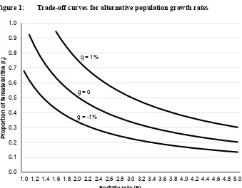
7. The trade-off between fertility and the sex ratio at birth
The stable population rate of growth can be thought of as determined by two parameters, the fertility rate and the proportion of female births (conditional on the early-life female mortality rates sf0 and sf1). Manipulating the equation for the growth rate in section 4 we may write it in the alternative form ln(1+g)=
f
r F
H+.025ln +.025ln , where the constant H =.025(lnsf0+lnsf1). The possibilities for trade-off between fertility and the female birth proportion are implicit in Table 4 but this form of the equation makes them explicit: for any given value of g the pairs of F
and rf that would yield that rate can be calculated. Trade-off curves of this kind are
shown in Figure 1 for g =−1%,0%,1%, for illustration. The horizontal axis in the figure represents F, the vertical axis rf , and the points on a curve the alternative combinations of F and rf that would yield the given growth rate. A stationary
Figure 1: Trade-off curves for alternative population growth rates
8. Alternative survival rates and the rate of growth
We have calibrated the Q matrix by assigning to it a particular set of survival rates. A different set would have little effect on the results. The results that we derive for a stable population depend critically on the fertility rate and the male/female proportions at birth: they are relatively insensitive to the choice of survival rates. We illustrate that now by recalculating some of the stable population growth rates in Table 4 with death rates increased by multiples of two, five, and ten, and the associated survival rates reduced accordingly.
As shown earlier, the annual population growth rate is given by 1
)
( 1/40
0
1 −
= s s r F
g f f f so that the only two survival rates that affect the stable growth
rate are sf0 and sf1. We now lower these survival rates by assuming that the corresponding death rates increase by a factor K. A survival rate s is thus replaced by
0.0 0.1 0.2 0.3 0.4 0.5 0.6 0.7 0.8 0.9 1.0
1.0 1.2 1.4 1.6 1.8 2.0 2.2 2.4 2.6 2.8 3.0 3.2 3.4 3.6 3.8 4.0 4.2 4.4 4.6 4.8 5.0
Pr
opor
tion of
fe
m
al
e
bi
rt
hs
(rf
)
Fertility rate (F) g = 1%
g = 0
) 1 (
1 K s
s∗= − − . We choose four alternative K values: K=1,2,5,10. Both survival
rates are adjusted in this way and the resulting growth rates are shown in Table 5 for alternative combinations of m/ f and F. To show the limits of the effects of the recalculations we choose the combinations at the four corners of the growth rate panel in Table 4, i.e., the four combinations of m/f =1.05 or 1.45 with F=1.0 or 5.0. As in Table 4, the growth rates are expressed in percentage form.
Table 5: Effects of higher mortality on the annual rate of growth in a stable Alpha population: death rates increased for female births and female children
Percent growth when death rates increased by factor K
F m/f K = 1 K = 2 K = 5 K = 10
1.000 1.05 -1.808 -1.837 -1.926 -2.078
1.000 1.45 -2.244 -2.273 -2.362 -2.513
5.000 1.05 2.224 2.193 2.101 1.943
5.000 1.45 1.769 1.739 1.647 1.490
Note: See text for the basis of the calculations in this table. When K = 1 there is no change in death rates and the growth rates are the same as in Table 4.
Setting K =1 means no change in survival rates, and hence stable population growth rates that are identical to those in Table 4. A two-fold increase in the death rates (K=2) changes the growth rates by no more than .031%, a five-fold increase (K=5) by no more than .123%. Even a ten-fold increase (K =10) changes the rates at most by .281%. The growth rates in Table 5 thus show very little sensitivity to changes in survival rates.
9. Summary and discussion
presence of sex-selective abortion the effect on the male/female proportions may be large, and other effects quite different from what they would otherwise be.
We began with a particular set of nine stopping rules, one with no male preference, two with male preference but no abortion, and six with male preference and the availability of abortion as an aid to achieving a desired number of male births. We calculated the probability distribution over the number of births and number of male births for each rule. We then assumed, for each, that it was adopted by all women bearing children, and worked out the effects that that would have on the population – in particular the effects on the male/female ratio at birth, the overall fertility rate, the age distribution of the population, the sex distribution at each age, and the rate of growth. We then changed course: we assumed that there were unspecified combinations of stopping rules that could generate particular fertility rates and male-biased sex ratios at the aggregate level, and calculated the effects that that would have on the population for a large number of combinations of the two. (Given a wide range of possible stopping rules, and potential heterogeneity in the choice of a rule within the population, there could in fact be a wide range of fertility/sex-ratio outcomes within our framework of analysis.)
of the fertility rate and birth sex ratio, as seen in the trade-off curves in Figure 1. The fifth observation is that the rate of population growth, in particular, is quite insensitive to the specification of survival rates, and in fact only the early-life rates for females matter (sf0, sf1). We calibrated our model with a given set of survival rates but changing those rates has little effect on the growth rate; growth is driven almost entirely by the fertility rate and male/female ratio at birth in our experiments.
It is not surprising that the ability to change the birth probabilities in favour of males has the types of effects just mentioned. What we would like to be viewed as the contribution of this paper is the analytical quantification of effects that might have been predictable in general, but which require model-based calculations to see how large they could in fact be. That has been our aim. In terms of the existing literature, we would like to think of the paper, with its emphasis on population effects, as a useful complement to the growing literature on sex-selective abortion and stopping rules at the family level, as noted in our introduction.
It is perhaps appropriate, in conclusion, to take note of some of the issues that we have not attempted to address. One thing the paper does not do is to consider the dynamics of adjustment – the process of moving from one stable state to another in a situation in which sex selection becomes more widely practised. Nor does it consider how an actual (as opposed to theoretical) population might evolve in such a situation, or the population implications of migration from a country or region in which sex selection is more common to one in which it is not. (See in that regard our references at the beginning of the paper.) How an increased ratio of males to females in the general population might itself come to influence future fertility choices is another question that could be put on the list, and more generally the societal consequences of an increased proportion of men in the population, and a decreased proportion of women. At an analytical level, we have assumed homogeneity of fecundity in specifying stopping rules, and common male/female probabilities at birth in the absence of sex-selective abortion, thus ignoring natural differences that may in fact exist in a population. Also, we have disregarded the role that child mortality might play in the application of stopping rules – the death of a son, say, which might alter preferences in regard to subsequent births. One can think too of other matters of possible relevance that play no role in our analysis. Having said that, we observe that all papers ignore some things in order to focus on others – and so it is with ours.
10. Acknowledgements
References
Abrevaya, J. (2009). Are there missing girls in the United States? Evidence from birth data. American Economic Journal: Applied Economics 1(2): 1–34. doi:10.1257/
app.1.2.1.
Almond, D. and Edlund, L. (2008). Son-biased sex ratios in the 2000 United States census. Proceedings of the National Academy of the United States of America
105(15): 5681–5682. doi:10.1073/pnas.0800703105.
Almond, D., Edlund, L., and Milligan, K. (2013). Son preference and the persistence of culture: Evidence from South and East Asian immigrants to Canada. Population
and Development Review 39(1): 75–95. doi:10.1111/j.1728-4457.2013.00574.x.
Bongaarts, J. (2013). The implementation of preferences for male offspring. Population
and Development Review 39(2): 185–369. doi:10.1111/j.1728-4457.2013.00
588.x.
Cohen, J.E. (1979). Ergodic theorems in demography. Bulletin of the American
Mathematical Society (New Series) 1: 275–293.
doi:10.1090/S0273-0979-1979-14594-4.
Cull, P. and Vogt, A. (1973). Mathematical analysis of the asymptotic behavior of the Leslie matrix model. Bulletin of Mathematical Biology 35(5–6): 645–661.
doi:10.1007/BF02458368.
Dubuc, S. and Coleman, D. (2007). An increase in the sex ratio of births to India-born mothers in England and Wales: Evidence for sex-selective abortion. Population
and Development Review 33(2): 383–400. doi:10.1111/j.1728-4457.2007.00
173.x.
Fuse, K. (2013). Daughter preference in Japan: A reflection of gender role attitudes?
Demographic Research 28(36): 1021–1052. doi:10.4054/DemRes.2013.28.36.
Goodman, L.A. (1961). Some possible effects of birth control on the human sex ratio.
Annals of Human Genetics 25(1): 75–81. doi:10.1111/j.1469-1809.1961.tb0
1500.x.
Guilmato, C.Z. (2010). Longer-term disruptions to demographic structures in China and India resulting from skewed sex ratios at birth. Asian Population Studies 6(1): 3–
Jiang, Q., Li, S., and Feldman, M.W. (2011). Demographic consequences of gender discrimination in China: simulation analysis of policy options. Population
Research and Policy Review 30(4): 619–638. doi:10.1007/s11113-011-9203-8.
Keyfitz, N. (1968). Introduction to the Mathematics of Population. Reading, Mass.: Addison-Wesley.
Keyfitz, N. and Caswell, H. (2005). Applied Mathematical Demography, Third Edition. New York: Springer.
Kintner, H.J. (2008). The life table. In: Siegel, J.S. and Swanson, D.A. (eds.). The
Methods and Materials of Demography, Second Edition. Bingley, UK: Emerald
Group Publishing Limited.
Livingston, G. and Cohn, D. (2010). Childlessness up among all women; down among women with advanced degrees. Pew Research Social and Demographic Trends, June 25, 2010.
Ray, J.G., Henry, D.A., and Urquia, M.L. (2012). Sex ratios among Canadian liveborn infants of mothers from different countries. Canadian Medical Association
Journal 184: E492–E496. doi:10.1503/cmaj.120165.
Statistics Canada (2006). Life tables, Canada, provinces and territories 2000 to 2002. Ottawa. Catalogue 84-537-XIE.
Yadava, R.C., Kumar, A., and Srivastava, U. (2013). Sex ratio at birth: A model based approach. Mathematical Social Sciences 65(1): 36–39. doi:10.1016/j.mathsocsci.
2012.06.004.
Yamaguchi, K. (1989). A formal theory for male-preferring stopping rules of childbearing sex differences in birth order and in the number of siblings.