Prediction of soil cation exchange capacity using support vector regression optimized by genetic algorithm and adaptive network-based fuzzy inference system

(1)

DESERT

Desert

Online at http://desert.ut.ac.ir

Desert 22-2 (2017) 187-196

Prediction of soil cation exchange capacity using support vector

regression optimized by genetic algorithm and adaptive

network-based fuzzy inference system

H. Shekofteh

a*

, F. Ramazani

b

a

Soil Science Department, University of Jiroft, Jiroft, Iran b

Soil Science Department, University of Rafsanjan, Rafsanjan, Iran

Received: 3 March 2017; Received in revised form: 16 September 2017; Accepted: 25 September 2017

Abstract

Soil cation exchange capacity (CEC) is a parameter that represents soil fertility. Being difficult to measure, pedotransfer functions (PTFs) can be routinely applied for prediction of CEC by soil physicochemical properties that can be easily measured. This study developed the support vector regression (SVR) combined with genetic algorithm (GA) together with the adaptive network-based fuzzy inference system (ANFIS) to predict soil CEC based on 104 soil samples collected from soil surface under four different land uses. The database was randomly split into training and testing datasets in proportion of 70:30. The results showed that both models were accurate in predicting the soil CEC; however, comparison of the performance criteria indicated that SVR results (R2_{=0.84, RMSE=3.21 and}

MAPE=7.62) was more accurate than ANFIS results (R2_{=0.81, RMSE=3.38 and MAPE=10.31). The results of}

sensitivity analysis showed that two parameters had the highest effect on both models were soil organic matter and clay content.

Keywords: Soil cation exchange capacity; Support vector regression; ANFIS; Genetic algorithm; Soil physiochemical properties

1. Introduction

The soil cation exchange capacity (CEC) is defined as the number of the adsorbed cation charge moles that are desorbed from a unit mass of soil under specific conditions of temperature, pressure, soil solution composition, and soil solution (Sposito, 2008). CEC is commonly referred to as the quantity of negative charges in soil. The negative charge may be pH dependent (soil organic matter) or permanent (some clay minerals) (Evans, 1989). CEC is a good indicator of soil fertility, crop growth, and pollutant transport and determines the buffering capacity of a soil to hold the cationic nutrients and organic pollutants (Arias et al., 2005; Tang

et al., 2009; Visconti et al., 2012) and is therefore an important parameter for prediction



Corresponding author. Tel.: +98 913 3481945 Fax: +98 348 31312041

E-mail address: [email protected]

of crop yield. De la Rosa et al. (1981) found that CEC, carbonate content, salinity and sodium saturation were conducive to 78% of the variation in winter wheat yields. To estimate maize and soybean yields, Sharma et al. (2013) successfully applied regression models in which CEC was one of six explanatory variables. Different crop models like EPIC (Williams et al., 1989) and CropSyst (Stockle et al., 1994) make use of CEC as an important modeling parameter. Therefore, precise knowledge of CEC data helps determining the accuracy of crop yield simulation. In addition, through soil CEC, the rate of the absorption of different pollutants like diquat and paraquat (Delle Site, 2001), and atrazine or phenanthrene (Chung and Alexander, 2002) can be determined. Overall, a good understanding of soil CEC is important for crop, soil and environmental researches.

(2)

Shekofteh & Ramazani / Desert 22-2 (2017) 187-196 188

worth applying indirect methods for accurate prediction of CEC. Pedotransfer functions (PTFs) can be a method for predicting CEC from basic soil properties being more easily measured (Krogh et al., 2000; Seybold et al., 2005).

According to previous studies, clay and soil organic matter (SOM) contents strongly affect the capacity of a soil for buffer changes in pH (Syers et al., 1970; Oorts et al., 2003). Consequently, these physicochemical properties can be useful predictors for estimating the CEC of a soil (Horn et al., 2005; Tang et al. 2009). However, since PTFs developed by different methods have different results, the selection of the appropriate PTFs is difficult. Traditional PTFs have developed through multiple linear regressions (MLRs) or artificial neural networks (ANNs). Seybold et al. (2005) developed a MLR-based PTF for soil CEC and realized that the pH, SOM and clay content had a strong correlation with CEC. Moreover, soil structure, water content at permanent wilting point, hydraulic conductivity and soil horizons can be important predictors of CEC in soils (Madeira et al., 2003; Seybold et al., 2005; Tang et al. 2009). However, a disadvantage of regression models is that any equation is able to imitate only a particular shape of the dependence (Wösten et al., 2001).

Nowadays, support vector machines (SVMs) ― new learning algorithms― are becoming popular in a wide variety of pedological applications. SVM was first developed for classification purposes (Boser, 1992) and then extended for regression (Vapnik, 1995; Smola and Schölkopf, 1998). SVM is well-founded and theory-based in statistical learning (Vapnik, 1998). SVM implement the principal of structural risk minimization instead of experiential risk minimization (Shia et al., 2012). Therefore, SVM has an excellent generalization capability in the situation of small sample sizes. Lamorski et al. (2008) compared ANN and SVM to develop PTFs in order to predict soil water retention parameters for Polish soils. Here SVM was superior compared to ANN. Liao et al. (2014) compared performance of SVM models to multiple stepwise regression (MSR) and ANN models. Results showed that the accuracy of CEC predicted by SVM were higher compared to prediction by MSR and ANN. In addition, SVM has performed successfully in engineering (Dibike et al., 2001) and hydrological forecasting (Liong and Sivapragasam, 2002). In conclusion, SVM seems to be a promising tool

for the development of PTFs for CEC prediction.

Another tool used to develop a PTF for predicting soil parameters can be an adaptive network-based fuzzy inference system (ANFIS). ANFIS is a fuzzy rule-based system that uses ANNs theory to determine the parameters of the fuzzy membership functions. In ANFIS, both learning capabilities of a neural network and reasoning capabilities of fuzzy logic can be combined to enhance predictions compared to a single methodology. ANFIS is potentially able to model nonlinear functions. It learns features of the dataset and adjusts the system characteristics according to a given error criterion (Jang, 1993).

(3)

regression and ANN for prediction of CEC and found that the radial basis function neural net was more accurate than the other models but the accuracy of ANFIS and multiple layer perceptron neural net were better than multiple linear regression. To our knowledge, little research is available for using SVM and ANFIS for predicting soil CEC. The objectives of this study were therefore to derive ANFIS and SVM-based PTFs for predicting CEC of different land uses and to compare the predictive capabilities of the SVM model with ANFIS model.

2. Materials and Methods

2.1. Soil sampling and analysis

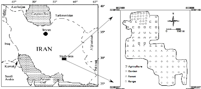
This study was conducted in some part of Rabor region (from 29 27′ N to 38 54′ N and 56 45′ E to 57 16′ E). The study area (400 ha) is located in the south-west part of Kerman province, Iran (Figure 1). Rabor is a typical semi-arid land farming area with a cold temperate climate. The annual mean temperature is 15 C with an average annual precipitation of 250 mm.

A total of 104 natural soil samples from four land uses were collected from the soil surface (0-15 cm). Land uses included garden with 20 year-old walnut trees, pasture, agriculture and forest of mountain almond.

A total of 104 natural soil samples from soil surface (0-15 cm) of four land uses were collected. Land uses included gardens with 20 year-old walnut trees, pasture, agriculture and forest of mountain almond. A grid sampling strategy was designed using ILWIS 3.4 software (ITC, University of Twente, the Netherlands)

for a proper selection of soil sampling locations to consider spatial variations of the parameters influencing the soil CEC in the study area. At each sampling point, disturbed and undisturbed samples were taken. For disturbed soil samples large plant materials (i.e., roots and shoots) and pebbles in each sample were separated by hand and discarded. The positions of the sampling points were identified in the field using GPS (model 76 CSx, Garmin Co., Taiwan). The disturbed soil samples were air-dried and ground to pass a 2 mm sieve. Soil organic matter (SOM) content was determined by the Walkley–Black method with dichromate extraction and titrimetric quantization (Nelson and Sommers, 1982). Percentages of clay (>0.002 mm), silt (0.002–0.05 mm), and sand (0.05–2 mm) particles were measured by means of the sieving and sedimentation method (Gee et al., 1986). Soil particle density (PD) using Blake and Hartge (1986) method , and calcium carbonate equivalent (CCE) was determined by the back-titration method (Nelson and Sommers, 1982). Soil pH was measured in saturated paste using a digital pH-meter (Model 691, M0065trohm AG Herisau, Switzerland) (Rhoades et al., 1996), electrical conductivity (ECe) was determined in the extract using an electrical conductivity meter (Model Ohm-644,Metrohm AG Herisau, Switzerland) (Rhoades et al., 1996), and CEC using sodium acetate (pH= 8.2) (Thomas, 1982). Undisturbed soil samples were taken at each location using 100 cm3_{core samples and were used to} determine the soil bulk density (BD) based on the core method (Klute, 1986). Porosity was calculated by the relation of bulk density and particle density.

(4)

2.2. Support vector machines and genetic algorithm

SVM, first proposed by Boser et al. (1992), is a training algorithm for classification and regression problems. In the case of regression (support vector regression, SVR), initially, a mapping from input space onto a high-dimensional feature space is performed. Then, a linear regression is performed through a hyperplane in the feature space by 𝜀-insensitive loss. Via a kernel function, SVR provides a mechanism that fits the hyperplane surface to the training data. To make a point, setting of kernel parameters is vital because this can add to the accuracy of the SVR prediction. For more information we refer to the theory of support vector regression in (Vapnik, 2013). In our work, we used radial basis function (RBF) as kernel function. Contents of SOM, sand, silt, clay, calcium carbonate and the pH value were chosen as the inputs to the RBF-based SVR with CEC as the output. The data set included the sampled 104 points and was randomly divided into two datasets, a training dataset and a testing dataset at a ratio of 70:30. The former (73 soil samples) was used for developing the SVR and the latter (31 soil samples) for testing the performance of the developed SVR. SVR computations were performed by the MATLAB programming language. The SVR parameters known as the penalty parameter, C, the width parameter, 𝛾, for the RBF kernel, and the variable 𝜀 are all required for SVR training (Wohlberg et al., 2006). We obtained the parameters by genetic algorithms (GA). As a general adaptive optimization search based on a direct analogy to Darwinian natural selection and genetics in biological systems, GA can efficiently cope with large search spaces. In this study, real-valued GAs (RGAs) were used. Definition of the objective function is the first step to apply GA and the value of objective function for each individual is usually used as a measure of the individual’s fitness. In this study, in order to avoid the variable scale, the relative mean absolute percentage error (RMAPE) was considered as the main objective. The objective function and fitness function are defined as follows:

Objective function=

RMAPE= ₎ ₁₀₀

) (

) ( ) ( 1 (

1 







n i

i i i

o Y

o Y p Y

n

(1)

Fitness function=100- RMAPE (2)

Where Y(pi) and Y(oi) are observed and predicted values of CEC respectively and n

(104) is the number of data.

In a GA, a population of points (solutions) is first generated randomly. For every chromosome in the population, the fitness is computed. Here, a fitness-proportionate method also called roulette wheel selection (Michalewicz, 1994) is utilized to select individuals for reproduction based on their fitness values. After parent selection, the genetic operation of crossover is performed on each mated pair with a certain probability, referred to as crossover probability. The common crossover operations can be uniform, single-point, two-points, and arithmetic crossover (Michalewicz, 1994). For a RGA, arithmetic crossover is simple and effective. Here we selected and designed an arithmetic crossover for the crossover operation. In the next step, a mutation operation was applied. A Gaussian mutation was selected and designed to the mutation operation. After the produce of next generation (offspring), stopping criteria was checked and the algorithm was repeated until a specified termination criterion such as a limit in the maximum number of generation or no obvious change of fitness or preset fitness was satisfied. We tried different values for GA parameters in order to find the best parameters.

2.3. ANFIS

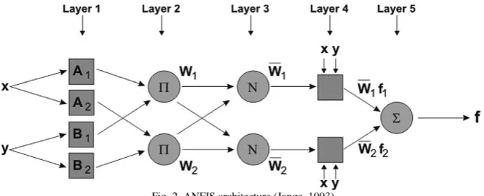
ANFIS is a multilayer feed-forward network in which each node performs a particular function on incoming signals as well as a set of parameters related to this node (Jang, 1993). Like ANN, ANFIS is able to learn the rules from previously seen data and thus map the unseen inputs to their outputs. This type of network can be simplified to a structure having two inputs of x and y and one output of f only as shown in Figure 2. From the Figure it can be seen that the architecture of ANFIS contains five layers, fuzzify, product, normalized, defuzzify and a total output layer. By assuming two membership functions for each of the input data x and y the general form of a first-order TSK (Takagi and Sugeno, 1985; Sugeno and Kang, 1988) type of fuzzy if–then rule can be described as

Rule i: IFx is Ai and y is Bi THEN

i i i

i

p

x

q

y

r

(5)

Where n is the number of rules and Pi, qi and ri

are the parameters determined during the training process.

In ANFIS, the inputs and output and the data for training and testing were the same as SVR. The data set was randomly divided into two smaller sets: a training data set (73 data points) and a testing data set (31 data points). The aim of the training process was to minimize the error between the actual target and ANFIS output. This allows ANFIS to learn features observed from the training data and then implement them in the system rules. In the performance phase,

the test data was introduced into the learned system for evaluation. A test error having an adequately small value indicated that the system showed a good generalized capability. The model was implemented in MATLAB (2014) software. The selection of rules in ANFIS is automatic and based on the data as we did it. In ANFIS, membership functions should be soft and of derivative type. We tried different soft membership functions and finally Gaussian membership functions was selected as membership function.

Fig. 2. ANFIS architecture (Jange, 1993)

2.4. Evaluation criteria

The predictive capabilities of the proposed models were evaluated by the root mean square error (RMSE), coefficient of determination (R2_), and mean absolute percentage error (MAPE) between measured and predicted values. The MAPE, RMSE and R2_{are denoted as below:}

1

( ) ( )

1

100 ( )

n i i

i

Y p Y o

MAPE

n  Y o

  

_ _







(4)

 

2 1

1 n i

RMSE Y pi Y oi

n _





_  _ (5)

1

2

2 2

1

( ( ) )( ( ) )

( ( ) ) ( ( ) )

n

i i

i n

i i

i

Y p Y p Y o Y o

Y p Y p Y o Y o

R 



 _

 

    

  _

 



(6)

Where Y(pi) and Y(oi) are the measured and predicted soil CEC values respectively, Yp and

Yo are the means of measured and predicted soil CEC values, and n is the total number of observations.

3. Results and Discussion

3.1. Statistical analysis of data

(6)

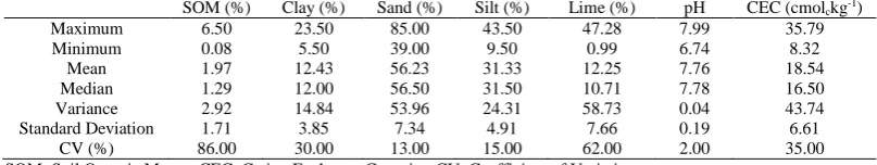
Table 1. Traditional statistics of physicochemical properties of soils under studied area

SOM (%) Clay (%) Sand (%) Silt (%) Lime (%) pH CEC (cmolckg-1)

Maximum 6.50 23.50 85.00 43.50 47.28 7.99 35.79

Minimum 0.08 5.50 39.00 9.50 0.99 6.74 8.32

Mean 1.97 12.43 56.23 31.33 12.25 7.76 18.54

Median 1.29 12.00 56.50 31.50 10.71 7.78 16.50

Variance 2.92 14.84 53.96 24.31 58.73 0.04 43.74

Standard Deviation 1.71 3.85 7.34 4.91 7.66 0.19 6.61

CV (%) 86.00 30.00 13.00 15.00 62.00 2.00 35.00

SOM: Soil Organic Matter, CEC: Cation Exchange Capacity, CV: Coefficient of Variation

3.2. SVR

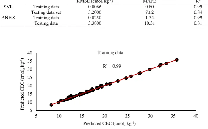
When training SVR, the optimum parameters 𝜀, C, and 𝛾 were found by a genetic algorithm approach. GA properties for optimizing RBF-SVR parameters are shown in Table 2. The best SVR parameters were obtained with restrictions of 0.001 ≤ 𝜀 ≤ 100, 0 ≤ C ≤ 100, and 0.0001 ≤ 𝛾 ≤ 1000. SVR model was then derived from these parameter restrictions in order to predict CEC from the different land uses. The R2 (Figure 3), RMSE and MAPE between SVR data and the measured data for training data were 0.99, 0.0066 cmolc kg-1 and 0.8 respectively. Based on these results, combination of SVR with GA can lead to an accurate understanding of the connections between the input and output data. There is proof that genetic algorithms are effective and robust tools for solving optimization problems (Davis, 1991). The performance criteria values for testing data are shown in Table 3. The R2 (Figure 4), RMSE and MAPE for testing data were 0.84, 3.2 cmolc kg-1 and 7.62 respectively. These values are indicative of the capability of SVR model for prediction of soil CEC in the studied area.

SVR is efficient for solving small sample size problem since it tends to avoid local minima that ANFIS usually suffers from. Lamorski et al. (2008) also found that the SVR provided the same or better accuracy compared with ANN in the prediction of soil water characteristics. Due to large heterogeneity in the CEC of natural soils, prediction of large-scale CEC is difficult. Hence, for large-scale crop modeling, SVR can provide an accurate estimation of CEC. Compared to other studies,

our results show that the SVR for prediction of soil CEC are comparable to or even superior to other studies, Sahrawat (1983) for soils in the Philippines, Bell and van Keulen (1995) for soils in Mexico, Seybold et al. (2005) for soils in North America, Ersahin et al. (2006) for soils in Turkey, Kalkhajeh et al. (2012) for soils in Iran, and Liao et al. (2014) for soils in China. In our study, the efficiency of GA method for searching optimal SVR parameters is proved. Previous studies have used other methods to obtain the optimal SVR parameters. Twarakavi

et al. (2009) used a grid-based SVM search approach. To them, this approach contributed to a significant improvement of prediction of soil hydraulic parameters compared with ANN-based ROSETTA.

3.3. ANFIS

The R2 _{between ANFIS and measured data} for training data was 0.99 (Figure 5). The RMSE and MAPE between ANFIS predicted data and measurement for training data were 0.025 cmolc kg-1. and 1.34 respectively. The results show that ANFIS can capture the relationship between the input parameters and soil CEC with a high accuracy. The performance criteria values for the test data are presented in Table 3. The R2 _{(Figure 6), RMSE} and MAPE values for testing data were 0.81, 3.38 cmolc kg-1 and 10.31 respectively. The values of performance criteria show that ANFIS model is a useful tool for predicting soil CEC. Kashi et al. (2014) and Ghorbani et al. (2015) also reported accuracy of ANFIS in predicting soil CEC is high.

Table 2. Values of GA parameters for obtaining SVR model parameters

Parameter Value

Crossover probability 0.7

Mutation probability 0.1

Number of generations 100.0

Number of variables 3.0

(7)

Fig. 3. The R2_{between measured and predicted cation exchange capacity (CEC) in the training dataset that were generated by SVR}

model

Fig. 4. The R2_{between measured and predicted cation exchange capacity (CEC) in the testing dataset that were generated by SVR}

model

Table 3. Values of performance criteria for SVR and ANFIS models

Model Evaluation criterion

RMSE (cmolc kg-1) MAPE R2

SVR Training data 0.0066 0.80 0.99

Testing data set 3.2000 7.62 0.84

ANFIS Training data 0.0250 1.34 0.99

Testing data 3.3800 10.31 0.81

R² = 0.99

5 10 15 20 25 30 35 40

P

re

d

ic

te

d

C

EC

(

cmo

lc

kg

-1)

Predicted CEC (cmolckg-1)

Training data

Fig. 5. The R2_{between measured and predicted cation exchange capacity (CEC) in the training dataset that were generated by}

(8)

R² = 0.81

5 10 15 20 25 30 35 40

M

ea

su

re

d

C

EC

(

cmo

lc

kg

-1)

Predicted CEC (cmolckg-1)

Testing data

Fig. 6. The R2_{between measured and predicted cation exchange capacity (CEC) in the testing dataset that were generated by ANFIS}

model

3.4. Sensitivity analysis of models

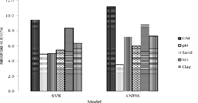
Results of the sensitivities of R2_{are shown in} Figure 7; for the SVR model, the sensitivities of R2_{corresponding to removals of OM, clay, silt,} sand, pH and calcium carbonate are 9.41%, 8,36%, 5.41%, 5.01%, 4.9%, and 6.35%, respectively while for ANFIS model the sensitivities are 11.18%, 8.9%, 6%, 7.2%, 3.5%, and 7.3%, in the same order of appearance. The figure shows that clay and OM had the most

effects on soil CEC respectively. As stated before, soil CEC represents negative charge amounts and the negative charge of soil was originated from clay and OM. Soil pH had the lowest effect on soil CEC in both models, as summary of descriptive statistical characteristics of physiochemical properties showed that the soil pH had the lowest coefficient of variation among all parameters thus it is reasonable that both models were less sensitive to the soil pH.

Fig. 7. The sensitivities of R2_{derived by SVR and ANFIS models to removals of soil physicochemical properties}

3.5. Comparison between SVR and ANFIS

Comparison of the obtained results from the proposed SVR and ANFIS models indicates that when predicting soil CEC the SVR technique is more feasible than the ANFIS model. On the other hand, the proposed SVR model in the current study was more effective in predicting the soil CEC than the ANFIS model when the performance criteria were compared. The R2

(9)

soil physicochemical properties in this area. SVR is efficient for solving the problem with a small number of samples and tended to avoid local minima that ANFIS usually suffers from them (Liao et al., 2014). Lamorski et al. (2008) also found that the SVR provided the same or better accuracy compared with ANN in the prediction of soil water retention characteristics. The main advantages of using SVRs are their flexibility and ability to model non-linear relationships. Furthermore, the SVR training process always seeks a global optimized solution and avoids over-fitting that eventually leads to better generalization performance than in ANFIS models. SVR is able to select the key vectors in the training process as its support vectors and remove the nonsupport vectors automatically from the model. This makes the model cope well with noisy conditions. The main disadvantage of the SVR and ANFIS techniques is that they have no physical basis and belongs to a class of data-driven black-box approaches.

4. Conclusions

This study was conducted to develop SVR and ANFIS-based PTFs for prediction of soil CEC in Rabor region of Kerman province, Iran. Although performance of both models was good, SVR was better than ANFIS. This suggests that SVR and ANFIS are robust tool for development of PTFs for CEC prediction. Sensitivity analysis showed that two parameters had the highest effect on both models were soil organic matter and clay content. These results obtained from a semiarid region in Iran so they could be applied to other parts of the world with similar challenges. In addition, due to soil, CEC is not a sit specific parameter; these methods could also be used in other parts of the world. It suggests these models compare to other techniques such as decision tree and artificial neural network.

References

Arias, M., C. Pérez-Novo, F. Osorio, E. López, B. Soto, 2005. Adsorption and desorption of copper and zinc in the surface layer of acid soils. Journal of Colloid and Interface Science, 288; 21-29.

Bell, M.A., H. Van Keulen, 1995. Soil pedotransfer functions for four Mexican soils. Soil Science Society of America Journal, 59; 865-871.

Besalatpour, A.A., S. Ayoubi, M.A. Hajabbasi, M.R. Mosaddeghi, R. Schulin, 2013. Estimating wet soil aggregate stability from easily available properties in a highly mountainous watershed. Catena, 111; 72-79.

Boser, B.E., I. Guyon, V. Vapnik, 1992. A training algorithm for optimal margin classifiers. In Fifth Annual Workshop on Computational Learning Theory, ed. D. Haussler. 144-152. New York: ACM Press.

Boser, B.E., E. Bernhard, M. Isabelle, I. Guyon, N. Vladimir,V. Vapnik, 1992. A training algorithm for optimal margin classifiers. In Proceedings of the fifth annual workshop on Computational learning theory, 144-152: ACM.

Chung, N., M. Alexander, 2002. Effect of soil properties on bioavailability and extractability of phenanthrene and atrazine sequestered in soil. Chemosphere, 48; 109-115.

De la Rosa, D., F. Cardona, J. Almorza, 1981. Crop yield predictions based on properties of soils in Sevilla, Spain. Geoderma, 25; 267-274.

Delle Site, A., 2001. Factors affecting sorption of organic compounds in natural sorbent/water systems and sorption coefficients for selected pollutants, A review. Journal of Physical and Chemical Reference Data, 30; 187-439.

Dibike, Y.B., V. Slavco, D. Solomatine, B.A. Abbott, 2001. Model induction with support vector machines: introduction and applications. Journal of Computing in Civil Engineering, 15; 208-216. Emamgolizadeh, S., S.M. Bateni, D. Shahsavani, T. Ashrafi, H. Ghorbani, 2015. Estimation of soil cation exchange capacity using Genetic Expression Programming (GEP) and Multivariate Adaptive Regression Splines (MARS). Journal of Hydrology, 529; 1590-1600.

Ersahin, S., H. Gunal, T. Kutlu, B. Yetgin, S. Coban, 2006. Estimating specific surface area and cation exchange capacity in soils using fractal dimension of particle-size distribution. Geoderma, 136; 588-597. Evans, LJ., 1989. Chemistry of metal retention by soils. Environmental Science & Technology, 23; 1046- 1056.

Gee, G.W., J.W. Bauder, 1986. Particle Size Analysis. In: Methods of Soil Analysis, Part A. Klute (ed.). 2 Ed., Vol. 9 nd . Am. Soc. Agron., Madison, WI, pp: 383-411.

Ghorbani, H., H. Kashi, N. Hafezi Moghadas, S. Emamgholizadeh, 2015. Estimation of Soil Cation Exchange Capacity using Multiple Regression, Artificial Neural Networks, and Adaptive Neuro- fuzzy Inference System Models in Golestan Province, Iran. Communications in Soil Science and Plant Analysis, 46; 763-780.

Horn, A.L., D. Rolf‐Alexander, G. Stefan, 2005. Comparison of the prediction efficiency of two pedotransfer functions for soil cation‐exchange capacity. Journal of Plant Nutrition and Soil Science, 168; 372-374.

Jang, J., 1993. ANFIS: adaptive-network- based fuzzy inference system. Systems, Man and Cybernetics. IEEE Transactions, 23; 665-685. Kalkhajeh, Y.K., R. Rezaie Arshad, H. Amerikhah, M. Sami. 2012, Comparison of multiple linear regressions and artificial intelligence-based modeling techniques for prediction the soil cation exchange capacity of Aridisols and Entisols in a semi-arid region. Australian Journal of Agricultural Engineering, 3; 39-40..

(10)

capacity based on multiple regression, ANN (RBF, MLP), and ANFIS models. Communications in Soil Science and Plant Analysis, 45; 1195-1213.

Klute, A., 1986. Methods of soil analysis. Part 1. American Society of Agronomy, Inc. Soil Science Society of America, Madison, Wisconsin, USA. Krogh, L., B.M. Henrik, H.G. Mogens, 2000. Cation- exchange capacity pedotransfer functions for Danish soils. Acta Agriculturae Scandinavica, Section B- Plant Soil Science, 50; 1-12.

Lamorski, K., P. Yakov, , C. Sławiński, R.T. Walczak, 2008. Using support vector machines to develop pedotransfer functions for water retention of soils in Poland. Soil Science Society of America Journal, 72; 1243-1247.

Liao, K., X. Shaohui, W. Jichun, L. Qing Zhu, 2014. Using support vector machines to predict cation exchange capacity of different soil horizons in Qingdao City, China. Journal of Plant Nutrition and Soil Science, 177; 775-782.

Liong, S.Y., S. Chandrasekaran, 2002. Flood stage forecasting with support vector machines1, ed.: Wiley Online Library.

Madeira, M., E. Auxtero, E. Sousa, 2003. Cation and anion exchange properties of Andisols from the Azores, Portugal, as determined by the compulsive exchange and the ammonium acetate methods. Geoderma, 117; 225-241.

Michalewicz, Z., 1994. GAs: What are they? In Genetic algorithms+ data structures= evolution programs, ed. 13-30: Springer.

Nelson, D.W., L.E. Sommers, 1982. Total carbon, organic carbon, and organic matter. Methods of soil analysis. Part 2. Chemical and microbiological properties (methodsofsoilan2); 539-579.

Oorts, K., B. Vanlauwe, R. Merckx, 2003. Cation exchange capacities of soil organic matter fractions in a Ferric Lixisol with different organic matter inputs. Agriculture, Ecosystems & Environment, 100 ; 161- 171.

Rhoades, J.D., 1996. Salinity: Electrical Conductivity and Total Dissolved Solids. In: Sparks, D.L., Page, A.L., Helmke, P.A., Loeppert, R.H., Soltanpour, P.N., Tabatabai, M.A., Johnston, C.T. and Sumner, M.E., Eds., Methods of Soil Analysis Part 3, Soil Science Society of America and American Society of Agronomy, Madison, pp: 417-435.

Sahrawat, K.L., 1983. An analysis of the contribution of organic matter and clay to cation exchange capacity of some Philippine soils. Communications in Soil Science & Plant Analysis, 14; 803-809.

Seybold, C.A., R.B. Grossman, T.G. Reinsch, 2005. Predicting cation exchange capacity for soil survey using linear models. Soil Science Society of America Journal, 69; 856-863.

Sharma, V.k., R.R. Daran, S. Irmak, 2013. Development and evaluation of ordinary least squares regression models for predicting irrigated and rainfed maize and soybean yields. Transactions of the ASABE, 56; 1361-1378.

Shekofteh, H., M. Afyuni, M.A. Hajabbasi, B.V. Iversen, H. Nezamabadi-pour, F. Abassi, F. Sheikholeslam, 2013. Nitrate leaching from a potato field using adaptive network-based fuzzy inference system. Journal of Hydroinformatics, 15; 503-515. Shia, J., D. Wangxiu, L. Yanxi, 2012. Early Warning

Model of Business Group Financial Risks Based on SVM. J. Inform. Comput. Sci., 9; 3813- 3820.

Smola, A., J., S. Bernhard, 1998. On a kernel- based method for pattern recognition, regression, approximation, and operator inversion. Algorithmica, 22; 211-231.

Sposito, G., 2008. The chemistry of soils: Oxford university press.

Stockle, C., O. Steve A. Martin, S. Campbell, 1994. CropSyst, a cropping systems simulation model: water/nitrogen budgets and crop yield. Agricultural Systems, 46; 335-359.

Sugeno, M., G.T. Kang, 1988. Structure identification of fuzzy model. Fuzzy sets and systems, 28; 15-33. Syers, J.K., A.S. Campbell, T.W. Walker, 1970. Contribution of organic carbon and clay to cation exchange capacity in a chronosequence of sandy soils. Plant and Soil, 33; 104-112.

Takagi, T., M. Sugeno, 1985. Fuzzy identification of systems and its applications to modeling and control. Systems, Man and Cybernetics, IEEE Transactions on, 15; 116-132.

Tang, L., Z. Guongming, F. Nourbakhsh, G. L. Shen, 2009. Artificial neural network approach for predicting cation exchange capacity in soil based on physico-chemical properties. Environmental Engineering Science, 26; 137-146.

Thomas, G.W., In: (Ed.), M, pp. 159-165. 1982. Exchangeable cations. In ethods of Soil Analysis, Part 2, monograph 9, ed. A. L. Page. 159-165. Madison, WI: ASA.

Twarakavi, N.K.C., J. Šimůnek, M.G. Schaap, 2009. Development of pedotransfer functions for estimation of soil hydraulic parameters using support vector machines. Soil Science Society of America Journal, 73; 1443-1452.

Vapnik, V., 1995. The Nature of Statistical Learning Theory. New York, USA: Springer.

Vapnik, V., 1998. Statistical learning theory, 1998, ed.^eds.: Wiley, New York. 2013. The nature of statistical learning theory: Springer Science & Business Media.

Visconti, F., J.M. De Paz, JL. Rubio, 2012. Choice of selectivity coefficients for cation exchange using principal components analysis and bootstrap anova of coefficients of variation. European Journal of Soil Science, 63; 501-513.

Williams, J.R., C.A. Jones, J.R. Kiniry, D.A. Spanel, 1989. The EPIC crop growth model. Transactions of the ASAE, 32; 497-0511.

Wohlberg, B., D.M. Tartakovsky, A. Guadagnini, 2006. Subsurface characterization with support vector machines. IEEE Transactions on Geoscience and Remote Sensing, 44; 47-57.

Wösten, J.H.M., Y.A. Pachepsky, W.J. Rawls, 2001. Pedotransfer functions: bridging the gap between available basic soil data and missing soil hydraulic characteristics. Journal of Hydrology, 251; 123- 150.