0 INTRODUCTION
As titanium alloys are increasingly used in ever widening fields of high-performance applications, classical manufacturing techniques are being applied to these high-tech materials. Commercially pure (CP) and near-CP alloys are a special case in this respect, because of their hexagonal close packed (HCP), α-phase crystalline structure. Although these materials generally exhibit good cold workability [1], their relevant mechanical properties are quite different to those of the traditional engineering materials they are replacing, which can pose a problem under mass production conditions.
A comprehensive theoretical investigation of the deformation behaviour of near-CP titanium alloys can be found in [2]. The primary difficulties for cold forming arise from the high level of anisotropy present in these materials, both in yielding and in work hardening.
Given the high price of the raw material and usually relatively low production volumes, numerical simulation can be a very useful tool in this field in helping to establish a reliable production process, both to determine the feasibility of a given process and to optimise the process parameters and tooling geometry beforehand, minimising the need for costly trial and error testing. There have been some attempts in recent years to develop bespoke constitutive models for HCP metals, as found in [3] to [5], however, a key feature of a numerical method applied in an industrial environment is the ability to identify the necessary material parameters promptly and with readily
available tests. Biaxial testing needed to determine the input parameters of these constitutive models does not fall into this category, thus the Barlat 1989 material model [6] is used, which allows for input data to be derived from uniaxial tensile testing, while still retaining moderate flexibility.
The relation of the data derived from the standard tensile test to the necessary input parameters is examined and a method for accommodating some
specifics of α-titanium plasticity in the Barlat
1989 material model is presented. The Barlat flow
potential exponent m is evaluated for α-titanium via a
parametric analysis of the standard Erichsen cupping test. From this, a full material characterisation method is defined and used on the near-CP alloy 1.2ASN from Kobe Steel. Finally the method is validated on an example of a deep drawn part.
1 PROPERTIES OF α-TITANIUM ALLOYS AND THE BARLAT 1989 MATERIAL MODEL
1.1 Plasticity of α-Titanium Alloys
As with all HCP materials, the crystalline structure
of α-titanium dictates some specifics in its plastic
response. The shape of the unit cell makes the material prone to texturing during the rolling process and causes the deformation modes to be dependent on the loading direction. The deformation mechanisms of HCP metals are dictated by the c/a ratio of the unit cell [7], α-titanium alloys exhibit a c/a ratio of 1.587, which is lower than the geometrically ideal ratio of 1.663. The slip systems active in this instance are the
Numerical Simulation of Cold Forming
of α-Titanium Alloy Sheets
Jurendić, S. – Gaiani, S. Sebastijan Jurendić1, * – Silvia Gaiani1,2
1 Akrapovič d.d., Slovenia
2 University of Modena and Reggio Emilia, Department of Materials Engineering, Italy
Despite the generally good cold workability of some α-titanium alloys, their relevant mechanical properties are quite different to those of traditional cold forming materials. The hexagonal close packed (HCP) crystal structure of α-titanium alloys results in a highly textured, highly anisotropic material that exhibits some specifics in its plastic response. A numerical simulation method using the Barlat 1989 material model has been developed to aid in forming tool development and process parameter determination. In order to account for the anisotropic hardening of the material, plastic strain ratios are input into the model as functions of plastic strain and an inversely determined, experimental strain hardening curve is used. The procedure for determining the input data from the tensile test is outlined and demonstrated on the α-titanium alloy 1.2ASN from Kobe Steel. The flow potential exponent m is evaluated via a parametric analysis of the Erichsen test and an appropriate value is determined. The forming limit diagram is adopted as a means for failure prediction and determined using the Nakajima method. Finally, the method is evaluated on an example of a deep drawn part with good correlation to the physical process.
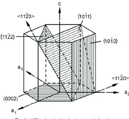
prismatic {1010} planes, the basal (0001) planes and the pyramidal {1011} planes, all in the basal direction <1210>. Together, they provide 4 independent slip systems that all occur in the basal direction, as a consequence a deformation system with a non-basal Burgers vector, such as <c+a> pyramidal glide or twinning, must be activated to accommodate an arbitrary plastic deformation (Fig. 1).
Fig. 1. HCP unit cell with slip planes and directions
The fundamental macroscopic plastic properties that follow from the HCP structure and make the material difficult to form are:
• high level of anisotropic yielding,
• high level of anisotropic hardening,
• yielding asymmetry.
Fig. 2. σ – ε curves in the longitudinal, diagonal and transverse direction typical for α-titanium
Yielding and hardening anisotropy are well
illustrated in the engineering σ – ε curves in the
longitudinal, diagonal and transverse directions, as shown in Fig. 2.
Yield stress increases significantly from the longitudinal to the transverse direction, while the hardening exponent n falls off, as does the elongation to ultimate tensile strength, although the total elongation stays roughly the same. Also noteworthy is the early and rather gradual onset of localized necking. The total post-necking deformation to break is extensive in the longitudinal direction, while in the transverse direction, the majority of the plastic deformation is achieved prior to necking necking. The yield asymmetry, also known as the strength differential (SD), is attributed to twinning being activated under compressive loading and is evident in the much lower yield point under compressive loading [8].
All this implies that the yield locus variation with plastic deformation is not only in size, but also in shape, and is asymmetrical with regard to the direction of loading. The former is evident also in the width to thickness plastic strain ratios:
Ri w
pl
tpl
=ε
ε , (1)
which have been found to exhibit a significant dependence on plastic strain, especially in the diagonal and transverse directions [9].
1.2 Barlat 1989 Material Model
The Barlat 1989 material model was chosen at this stage because its input parameters can be derived easily from the standard tensile test and have a well-defined physical relevance. The plane stress yield
criterion Φ is defined as:
Φ =a K K+ m+a K K− m+c K m= Ym
1 2 1 2 2 2 2σ ,(2)
where σY is the yield stress and K1 and K2 are defined
as:
K1= x 2h y
+
σ σ
, (3)
K2 x h y p xy
2
2 2
2
= −
σ σ + τ , (4)
a R
R R
R
= −
+ ⋅ +
2 2
1 0000 1
90
σx and σy are the stresses in the local x and y directions,
and a, c, h, p are material parameters:
c= −2 a, (6)
h R R R R = + ⋅ + 00 00 90 90 1
1 , (7)
and the p parameter is found by an iterative search
from the expression for the plastic strain ratio in an arbitrary direction φ (usually the diagonal direction is used):
R m Ym
x y ϕ ϕ σ σ σ σ = ∂ ∂ + ∂ ∂ − 2 1
Φ Φ . (8)
The flow potential exponent m determines the
base shape of the yield surface.
The material parameters a, h, c, p are directly
related to the R values in the longitudinal, diagonal
and transverse directions, thus if these values are input into the model as functions of plastic strain, the shape evolution of the yield locus can be taken into account.
The main drawback of this material model is that it cannot account for yield asymmetry in any way, however, it should still give adequate results for predominantly tensile load paths.
From the mathematical formulation described above, the necessary input data for the constitutive model are:
• plastic strain ratios as functions of true plastic
strain in three directions: R00, R45, R90 ,
• yield stress as a function of equivalent plastic
strain σ εY
( )
p in the longitudinal direction,• flow potential exponent m.
The first two are derived from the tensile test, the
exponent m, however, does require a biaxial test to
evaluate, but it should be similar for all materials with a common crystal structure.
2 ASN MATERIAL CHARACTERIZATION PROCEDURE
2.1 General Mechanical Properties of 1.2ASN
The general tensile properties were measured using the standard tensile test in accordance with the EN ISO 6892:2009 standard with the extensometer gauges at 80 mm. The sheet thickness was 0.9 mm. Five samples were tested in each direction, the values presented in Table 1 are average values of all the tests in their respective directions.
Table 1. General mechanical properties of 1.2ASN alloy
Dir. Elastic modulus [GPa] Yield strength [MPa] Tensile strength [MPa] Elongation at tensile strength [%] Elongation at break [%] 0° 107 323 457 18.4 32.1 45° 109 355 417 15.7 35.9 90° 109 394 437 9.0 34.5
2.2 Plastic Strain Ratios
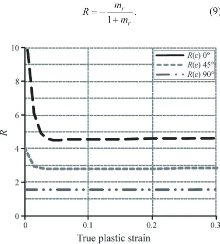
The plastic strain ratios as functions of true plastic strain should be determined first, as they are needed in the subsequent steps of the characterization procedure. The calculation procedure defined in the ISO 10113 standard [10] should be followed because of the large measurement error associated with plastic strain ratio measurement, especially at low strains [11]. The true plastic width strain should be plotted as a function of true plastic length strain and a linear regression fit through the data for the range of interest. The plastic strain ratio is calculated as follows from the slope of the linear regression mr:
R m
mrr = −
+
1 . (9)
Fig. 3. Plastic strain ratios as functions of true plastic strain in the longitudinal, diagonal and transverse direction
The plastic strain ratios are determined at intervals of 1% true plastic strain from initial yield to the onset of localized necking. From that point on the curves, high strains are manually extrapolated using
linear extrapolation. Fig. 3 shows the final R values
The variation in the longitudinal direction is nearly negligible while in the diagonal and transverse directions there is a significant initial variation before the values stabilize.
2.3 Yield Curve Determination
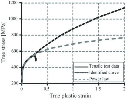
In contrast to steel, titanium exhibits substantial additional elongation past the point of localized necking with a fairly gradual onset of localization, which is not captured well by any of the traditional hardening laws, thus an experimental true stress-true strain curve was identified using an inverse procedure proposed in [12]. The yield curve is identified iteratively by running numerical simulations of the tensile test and by modifying the yield curve until an acceptable fit between the simulation and the tensile test is achieved. A fit within the scatter between samples of the same batch can be achieved without difficulties.
For this determination a ¼ symmetry model of the parallel section of the tensile specimen was modelled using shell elements. An element size of approximately 0.8 mm was adopted, as it is representative of the element sizes typically used in later forming simulations. Mass scaling was used to
maintain a time step of 5·10–7 and the deformation
rate was scaled by an order of 103, as this was found to
yield satisfactory results.
Fig. 4. Inversely identified yield curve, the power law approximation and the tensile test results
The final identified yield curve for 1.2ASN is shown in Fig. 4, along with the measured true stress-true strain curve and the functional approximation using a power law. Compared to the power law approximation it is much steeper at high strains, in order to support the extensive post-Rm deformation.
2.4 Calculation of Barlat 1989 Material Model Parameters
The a, c, h and p parameters of the Barlat 1989
material model are generally calculated internally in the numerical simulation software from the plastic strain ratios. Since the plastic strain ratios are functions of plastic strain, the Barlat parameters follow suit. Fig. 5 shows the a, h and p parameters as functions of true plastic strain.
The c parameter is not included in the graph,
as it is derived from the a parameter using simple
subtraction (Eq. (6)).
Fig. 5. Parameters of the Barlat 1989 material model
2.5 Flow potential exponent m
To determine an appropriate value for the m exponent,
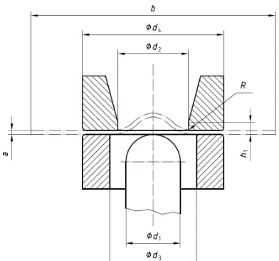
a parametric analysis was done using the Erichsen cupping test, as defined in the ISO 20482 standard (Fig. 6). In the absence of a viscous pressure bulge test, this test is a suitable alternative for this evaluation as it strains the material with biaxial tension, thus avoiding any SD effects, which pose a problem for the Barlat 1989 material model.
A numerical model of the Erichsen test was built and the input data determined above were used to run the simulations while varying the m parameter. The model is constructed from shell elements, with an average element size of approximately 0.7 mm in the deformation zone. The tools are considered to be rigid. A penalty contact formulation was used for the blank to tooling interfaces with a friction coefficient of 0.2.
Mass scaling to a time step of 1·10–6 was applied
force-displacement curves from the simulation were compared to the test results (Fig. 7).
Fig. 6. Schematic of the Erichsen test tooling
Fig. 7. Erichsen cupping parametric analysis results
The evaluation shows very good agreement for
m = 2. The anomalies in the curves above 7 mm of
displacement are attributed to contact instabilities, however, they do not affect the clarity of the results.
2.6 Friction Coefficient Determination
The frictional conditions between the blank and the tooling have a major effect on deep drawing processes. In order to evaluate the appropriate values of the friction coefficients, a series of wear tests were performed using a CSM pin-on-disc tribometer, according to the ASTM G99-05 (2010) standard. In this test, a disc of the test material rotates under a X100 Cr 6 steel pin with a hardness of 58 HRC. Two different pin geometries were used, a spherical
pin and a flat pin with a contact area of 1 mm2. The
linear pin speed was 15 cm/min, which is in the same order of magnitude as experienced under deep drawing, and the normal load applied to the specimen was 5 N. The duration of the tests was 30 min and the friction coefficient is the average value of the entire test, excluding the initial discontinuities typical of this method.
Combinations of available lubrication conditions were examined and the results are presented in Table 2.
Table 2. Friction coefficients under different lubrication conditions
Lubricant Type of pin μ
/ Spherical 0.45
/ Flat 0.50
Oil Spherical 0.44
Oil Flat 0.50
PVC foil unlubricated Flat 0.38 PVC foil + oil Flat 0.16 PVC foil + grease Flat 0.17
3 LIMITS OF FORMABILITY
As the goal of the simulation is to ultimately determine the feasibility of a given deformation process, the forming limit diagram (FLD) was determined for the material. The Nakajima method according to ISO 12004-2 [13] was used with optical strain measurement [14].
The test is based on deforming sheet metal samples of different geometries (Fig. 8) using a hemispherical punch up to the point of fracture.
Fig. 8. Nakajima test specimen geometries
Different strain paths are achieved by varying the width of the samples and each strain state at fracture
corresponds to a point on the major strain – minor
strain plot.
direction, for a total of 42 tests. The resulting forming limit diagram is shown in Fig. 9.
Fig. 9. Forming limit diagram for 1.2ASN
4 SIMULATION OF A DEEP DRAWN PART
4.1 Physical Part and Numerical Model
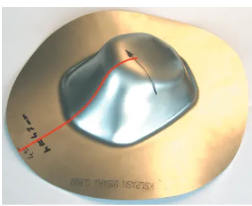
A motorcycle exhaust end-cap was selected for the simulation. It is a problematic shape to form with its tapering sides and a small top radius. This particular part cannot be drawn from the 1.2ASN material, the material fractures at the leading edge of the punch (Fig. 10). This allows for better evaluation of the method as the limits of formability are surpassed.
A series of drawing tests were carried out with longitudinal and transverse material orientations with regard to the longer axis of the end-cap. The maximum safe drawing depth was established to be 47 mm (the full depth is 90 mm). The thickness distribution was then measured on these samples along the line shown in Fig. 11.
Fig. 12 shows the numerical model of the end-cap deep drawing process. The model is comprised of three- and node shell elements, only four-node elements are used for the deformable blank and the average initial element size is approximately 4.5 mm. Adaptive remeshing of the blank is adopted, to a minimum element size of 0.9 mm.
Fig. 10. The part after failure
Fig. 11. The end-cap drawn to 47 mm with the thickness distribution measurement line
Fig. 12. End-cap drawing process numerical model
Mass scaling to a maximum time step of 1·10–6 is
used along with time scaling of the punch kinematics by a factor of about 500.
4.2 Results
The in-plane strains at 47 mm of drawing depth were plotted on the FLDs for the longitudinal and transverse direction (Figs. 13 and 14). They clearly show the localized deformation in the uniaxial strain region of the FLD that exceeds the forming limit curve. Those points coincide with the leading edge of the punch where fracture occurs.
Fig. 13. Minor – major strain plot for the longitudinal blank orientation at 47 mm of punch displacement
Fig. 14. Minor – major strain plot for the transverse blank orientation at 47 mm of punch displacement
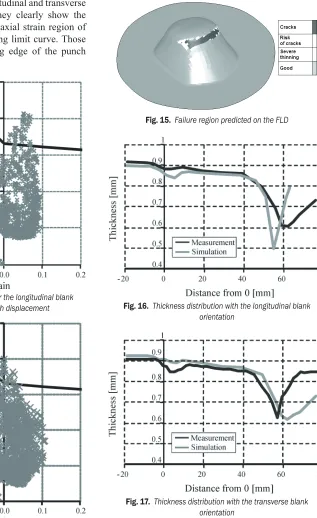
The simulations predict material fracture on the FLD at around 40 mm of depth for the longitudinal orientations and around 42 mm for the transverse orientation, which is somewhat conservative, however, both the location and shape of the predicted fracture compare well to the actual failed part (Fig.15).
Fig. 15. Failure region predicted on the FLD
Fig. 16. Thickness distribution with the longitudinal blank
orientation
Fig. 17. Thickness distribution with the transverse blank
orientation
depth were compared to the experimental thickness distributions measured on the actual parts. The zero point on the horizontal axis corresponds to the die shoulder, with the distance measured along the surface of the part. Figs. 16 and 17 show the results of the comparison.
The simulated thickness distributions compare fairly well to the measurements; the severe discrepancy in the longitudinal direction is due to the simulation predicting a break in the rosette before this depth is achieved. In both cases the simulated thickness lies below the measured distribution up to the point of local failure; it is suspected that the initial sheet might have been somewhat over-gauge.
Overall the results compare well with the actual process even if fracture is predicted prematurely, this might also have to do with the actual thickness of the sheet being slightly more than the nominal thickness used in the simulations.
5 CONCLUSIONS
Despite the inherent limitations of the Barlat 1989 material model with regard to the specifics of HPC materials, the simulation results show that this method is entirely adequate for running simulations at this level. The results correlate reasonably well with the experimental data, although the simulation is somewhat conservative. The cause of this could be the lack of strain-rate effects modelling, as the hardening curve is derived directly from the tensile test at low strain rates.
The procedure for acquiring the input data has proved to be robust and reliable in an industrial environment. Its primary drawback is that the inverse curve fitting procedure is time consuming and requires manual alterations to the yield curve between iterations, unless specialized optimization software is used.
While the parametric analysis of the Erichsen cupping test does provide a seemingly conclusive result, a better controlled biaxial stress test is still required to confirm the results. Such a test would provide a definite point on the yield locus that would
allow the accurate determination of the m exponent.
6 REFERENCES
[1] Lutjering, G., Williams, J.C. (2007). Titanium, 2nd ed. Springer, Berlin. Heidelberg, New York.
[2] Nixon, M.E., Cazacu, O., Lebensohn, R.A. (2010). Anisotropic response of high-purity α-titanium: Experimental characterization and constitutive modelling. International Journal of Plasticity, vol. 26, p. 516-532., DOI:10.1016/j.ijplas.2009.08.007.
[3] Plunkett, B., Lebensohn, R.A., Cazacu, O., Barlat, F. (2006). Anisotropic yield function of hexagonal materials taking into account texture development and anisotropic hardening. Acta Materiala, vol. 54, p. 4159-4169, DOI:10.1016/j.actamat.2006.05.009.
[4] Cazacu, O., Plunkett, B., Barlat, F. (2006). Orthotropic yield criterion for hexagonal close packed metals. International Journal of Plasticity, vol. 22, p. 1171-1194, DOI:10.1016/j.ijplas.2005.06.001.
[5] Lee, M.G., Wagoner, R.H., Lee, J.K., Chung, K., Kim, H.Y. (2008). Constitutive modelling for anisotropic/ asymmetric hardening behaviour of magnesium alloys sheets. International Journal of Plasticity, vol. 24, p. 545-582, DOI:10.1016/j.ijplas.2007.05.004.
[6] Barlat, F., Lian, J. (1989). Plastic behaviour and stretchability of sheet metals, Part 1: A yield function for orthotropic sheets under plane strain conditions. International Journal of Plasticity, vol. 5, p. 51-66, DOI:10.1016/0749-6419(89)90019-3.
[7] Wang, Y.N., Huang, J.C. (2003). Texture analysis in hexagonal materials. Materials Chemistry and Physics, vol. 81, p. 11-26, DOI:10.1016/S0254-0584(03)00168-8.
[8] Lissenden, C.J., Doraiswamy, D., Arnild, S.M. (2007). Experimental investigation of cyclic and time-dependent deformation of titanium alloy at elevated temperature. International Journal of Plasticity, vol. 23, p. 1-24, DOI:10.1016/j.ijplas.2006.01.006.
[9] Chamanfar, A., Mahmudi, R. (2005). Compensation of elastic strains in the determination of plastic strain ratio (R) in sheet metals. Materials Science and Engineering, vol. 397, p. 153-156, DOI:10.1016/j.msea.2005.02.039. [10] International Standard ISO 10113 (2006). Metallic
materials – Sheet and strip – Determination of plastic strain ratio. International Organization for Standardization, Geneva.
[11] ASTM Standard E 517-00 (2000). Standard Test Method for Plastic Strain Ratio r for Sheet Metal. ASTM International, West Conshohocken.
[12] Koc, P., Štok, B. (2008). Usage of the yield curve in numerical simulations. Strojniški vestnik - Journal of Mechanical Engineering, vol. 54, p. 821-829.
[13] International Standard ISO 12004-2 (2008). Metallic materials – Sheet and strip – Determination of forming limit curves Part2: Determination of forming limit curves in the laboratory. International Organization for Standardization, Geneva.