of peer-reviewed research and commentary in the population sciences published by the Max Planck Institute for Demographic Research Konrad-Zuse Str. 1, D-18057 Rostock · GERMANY www.demographic-research.org
DEMOGRAPHIC RESEARCH
VOLUME 12, ARTICLE 7, PAGES 141-172
PUBLISHED 14 APRIL 2005
www.demographic-research.org/Volumes/Vol12/7
DOI: 10.4054/DemRes.2005.12.7
Research Article
A comparison of different methods for
decomposition of changes in expectation of
life at birth and differentials in life
expectancy at birth
Krishna Murthy Ponnapalli
1 Introduction 142
2 A comparison of different methods 143 2.1 Chandra Sekar (1949) method 143 2.2 Arriaga’s (1984) method 148 2.3 Lopez and Ruzicka’s (1977) method 153 2.4 Pollard’s (1982) method 158 2.5 United Nations (1982) method 159 2.6 United Nations (1985) method 161
3 Conclusions 162
4 Acknowledgements 163
References 164
Appendix I 167
A comparison of different methods for decomposition of changes in
expectation of life at birth and differentials in life expectancy at birth
Krishna Murthy Ponnapalli1
Abstract
Several methods have been proposed to decompose the difference between two life ex-pectancies at birth into the contributions of diverse age groups. This study attempts to compare the system adopted by Chandra Sekar (1949) with various other methodologies such as those suggested by Arriaga, Lopez and Ruzicka and Pollard. The aim is to show that all these techniques in their modified (symmetrical) form will produce the same re-sult as that of United Nations, Pollard, Andreev and Pressat. Finally, this study suggests that the symmetric formulae of the above methods be used to arrive at near precise results since the percentage contribution of the sum of interaction terms with respect to difference in the life expectancy at birth is found to negligible.
1PhD, Senior Lecturer, Department of Fertility Studies, International Institute for Population Sciences,
1. Introduction
An increase or decrease in life expectancy at birth might be due to the changes that take place in the mortality conditions of different age groups over a period of time. A number of decomposition techniques have been developed (see Chandra Sekar, 1949, Retherford, 1972, Lopez and Ruzicka, 1977, Pollard, 1982, United Nations, 1982, Arriaga, 1984, United Nations, 1985, Andreev, 1982, Pressat, 1985, Das Gupta, 1993, Pullum and Tan, 1992, Andreev et al., 2002, Canudas Romo, 2003, Vaupel and Canudas Romo, 2003) to assess the corresponding effect of mortality change on life expectancy at birth.
Each of these decomposition procedures uses different formulas and consequently, produces variable results. However it is necessary to point out the similarities and dis-similarities between the different approaches; Chandrasekaran (1986), Pollard (1988) and recently, Pullum and Tan (1992), Vaupel and Canudas Romo (2003) are among those who have already made such an attempt. I quote Shkolnikov et al. (2001:7): “The formulae for decomposition by Andreev and Pressat are exactly equivalent. Arriaga’s formula is written in a slightly different form, but it is essentially equivalent to the formulae by An-dreev and Pressat.” Juxtaposing their new method with that of Arriaga (1984) Vaupel and Canudas Romo (2003) also conclude that “Arriaga’s method for decomposing change in life expectancy by age yields the same results as the Vaupel-Canudas method for Sweden around 1998.”
Chandrasekaran (1986) compared the procedures suggested by Pollard (1982), United Nations (1982), and United Nations (1985) with that of his own (Chandra Sekar, 1949) while Pollard (1988) contrasted the discrete approach of Arriaga (1984) with his own con-tinuous one (Pollard, 1982). Though the results of these two studies are interesting I feel there is also a need to look at Arriaga’s (1984), and Lopez and Ruzicka’s (1977) reports and scrutinize them in the context of all these other methods. This study is therefore an attempt to take forward the process of analyzing different decomposition procedures. In doing so the report also tries to extend the methodologies suggested by Chandra Sekar (1949), Arriaga (1984), Lopez and Ruzicka (1977) and Pollard (1982).
I list below the objectives of this study:
1. To describe and summarize the methods suggested by Chandra Sekar (1949), Lopez and Ruzicka (1977), Pollard (1982), Arriaga (1984), United Nations (1982) and United Nations (1985).
2. To extend the methodologies suggested by Chandra Sekar (1949), Arriaga (1984), Lopez and Ruzicka (1977) and Pollard (1982) and demonstrate that all four methods can be extended to give exactly the same results as that of United Nations (1985). 3. To demonstrate that decomposition formula in symmetric form of the method might
give more useful results than other forms of the method.
States from 1935 to 1995 (Box 3.4, P.65 of Preston et al., 2001). The data is reproduced here as Appendix Table 1. Here is a brief description of the notations used to describe each of the methods discussed below:
n m
1 x
= age specific death rate in the age group(x;x+n)in the initial
time period ‘1’
n m
2 x
= age specific death rate in the age group(x;x+n)in the latter
time period ‘2’ l
1 x
= number of persons alive at exact agex, in the initial time period ‘1’
l 2 x
= number of persons alive at exact agex, in the latter time period ‘2’
l 1 0
=l 2 0
= radix of the life table in the initial and latter time periods ‘1’ and ‘2’
e 1
x = expectation of life at exact age
x, in the initial time period ‘1’ e
2
x = expectation of life at exact age
x, in the latter time period ‘2’ n = length of the age interval.
In the present paper, for ease of computation, we shall assume thatl 1 0
=l 2 0
=1:0.
[Note: ‘1’ and ‘2’ may be taken as Male/Female, Urban/Rural, etc. in the study of differential mortality.]
In the following sections I have briefly described six methods suggested by different researchers and demonstrated that the modified version of Arriaga’s, Lopez and Ruzicka’s as well as Pollard’s approach – extended by following the Chandra Sekar (1949) method-ology – give identical results. Further, I have shown that Arriaga’s, Lopez and Ruzicka’s and even Chandra Sekar’s method in their modified form give exactly the same result as that of the United Nations (1985). The aim of my study is to bring these various method-ologies into the same picture, to provide a unified framework so to speak, and finally demonstrate that the United Nations (1985) method is the best among the ones in use not only because of its simplicity but also because it has been distilled from all the other methods.
Tables 1 to 4 and also Appendix Table 2 contain the result of the application of dif-ferent methodologies to the data on United States, females, from 1935 to 1995. This particular set of data was selected on the basis of its quality and accessibility (Preston et al., 2001:65).
2. A comparison of different methods
2.1 Chandra Sekar (1949) method
of effect – ‘main effect’, ‘operative effect’, interaction deferred’, and ‘effect-interaction forwarded’. All of these resulted from changes in mortality conditions in a specific age group during the two time periods considered. Chandrasekaran (1986: 2) defined the four effects thus:
Main effect: “The difference betweene 1 o
and the ‘expectation of life at birth which would have resulted’ if the mortality conditions had changed only in the age group under con-sideration to the extent that it had and the mortality conditions in the other age groups had remained unchanged”.
Operative effect: “The difference betweene 2
oand the ‘expectation of life at birth which
would have resulted’ if the mortality conditions had remained unchanged (or inoperative) in the specified age group and the mortality conditions in all other age groups had changed to the extent they had”.
Effect-interaction deferred: “The effect which would result if all interactions are as-signed to the oldest age group involved in its production”.
Effect-interaction forwarded: “The effect which would result if all interactions are as-signed to the youngest age group involved in its production”.
Chandrasekaran (1986:3) interpreted ‘interaction’ as effect “arising from mortality changes in two or more age-groups” and noted: “while the main effects ignore the ef-fect of interaction, each of the operative efef-fects takes it into account”. Chandrasekaran (1986:4) also gave the following formulae for measuring the four effects. These are ap-plicable to any age group ranging fromxtox+n.
Main effect =
l
1 x l
2 x
l 2 x
(e 2 x
e 1 x
) l 2 x+n
(e 2 x+n
e 1 x+n
) (1.1)
Operative effect =
l
2 x l
1 x
l 1 x
(e 2 x
e 1 x
) l 1 x+n
(e 2 x+n
e 1 x+n
) (1.2)
Effect-interaction deferred =
l 2 x
(e 2 x
e 1 x
) l 2 x+n
(e 2 x+n
e 1 x+n
) (1.3)
Effect-interaction forwarded =
l 1 x
(e 2 x
e 1 x
) l 1 x+n
(e 2 x+n
e 1 x+n
Chandrasekaran’s (1986) study compared his own method (Chandra Sekar, 1949) with the systems suggested by Pollard (1982), United Nations (1982) and United Na-tions (1985). The highlights of Chandrasekaran (1986:8) are:
1. “Pollard’s (1982) method includes both the main effect and interactions and tallies exactly with the values obtained by the United Nations (1985) method.”
2. “The value for the effect given in United Nations (1985) can be obtained by taking the average of the values for effect-interaction deferred and effect-interaction for-warded as given by Chandra Sekar (1949).”
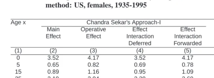
Analysis: First of all, Chandrasekaran’s (1986) comparative study failed to consider other important reports by Lopez and Ruzicka (1977), Arriaga (1984), Andreev (1982) and Pressat (1985). His investigation might well have been more interesting had he taken them into account, especially considering that one of his references is the United Na-tions (1982:135) work that alludes to the methodology suggested by Lopez and Ruzicka (1977). Secondly, though both his 1949 and 1986 studies discussed the ‘interaction terms’ in detail and suggested formulae for ‘Effect Interaction deferred” and “Effect Interaction forwarded”, they failed to suggest a formula for obtaining the ‘Total interaction effect’ as was done by Arriaga (1984) and Lopez and Ruzicka (1977). Thirdly, the method used in 1949 was not concise enough, though as Chandrasekarn (1986:8) said, and I quote, it “gives a range within which the effects lies”, probably for this reason his method is not used at all by other researchers. It was with this in mind that I tried to modify the method-ology originally suggested by Chandra Sekar (1949) because all things considered his was a brilliant attempt – no one else at the time had tried to explore this area of research. I would like to reiterate that this study’s attempt to unite the various methodologies is possible only because of Chandra Sekar’s 1949 work. Table 1 shows the results of the Chandra Sekar’s (1949) method applied to the data on United States females 1935-1995. The results in Table 1 are labeled Approach-I and Approach-II. According to Chan-drasekaran (1986:8) and as stated earlier both ‘effect interaction deferred’ and ‘effect interaction forwarded’ can be averaged to get the UN (1985) result. This is depicted in the study as Approach-II, and leads to the formula given below:
(e 2 x
e 1 x
)(l 2 x
+l 1 x ) 2
(e 2 x+n
e 1 x+n
)(l 2 x+n
+l 1 x+n
) 2
(1.5)
For the open-ended age group the above formula will be written as follows:
(e 2 x
e 1 x
)(l 2 x
+l 1 x ) 2
(1.6)
Table 1: Decomposition results obtained by using Chandrasekaran’s (1949) method: US, females, 1935-1995
Age x Chandra Sekar’s Approach-I Chandrasekaran’s
Main Operative Effect Effect Approach-II
Effect Effect Interaction Interaction
Deferred Forwarded
(1) (2) (3) (4) (5) (6) =[(4)+(5)]=2
0 3.52 4.17 3.52 4.17 3.85
5 0.65 0.82 0.69 0.78 0.73
15 0.89 1.16 0.95 1.09 1.02
25 2.19 2.94 2.39 2.69 2.54
45 2.73 4.02 3.18 3.43 3.31
65 2.89 4.58 4.07 3.26 3.66
85+ 0.26 0.88 0.88 0.26 0.57
Total 13.13 18.57 15.68 15.68 15.68
Source: Appendix Table 1
of Arriaga’s (i.e., Approach III) and Lopez and Ruzicka’s procedure (Approach III) and also as United Nations’ 1985 methodology.
Following Chandra Sekar, I tried to average the ‘two effects’ – the ‘main effect’ and ‘operative effect’ – and arrived at the formula given below:
(e 2 x
e 1 x
)(l 2 x
+l 1 x ) 2
(e 2 x+n
e 1 x+n
)
l 1 x l
2 x+n l
2 x
+ l
2 x l
1 x+n l
1 x
2
(1.7)
This formula (1.7) is presented as the ‘exclusive effect’ in the extended versions of Arriaga’s method (Approach III) and Lopez and Ruzicka’s method (Approach III).
Murthy and Gandhi (2004) suggested the following formula to work out the ‘Total interaction effect’ as obtained in Chandra Sekar’s (1949) method. This formula is realized by calculating the difference between ‘Total effect’ and ‘Exclusive effect’:
(e 2 x+n
e 1 x+n
) 0 B @
l 1 x l
2 x+n l
2 x
+ l
2 x l
1 x+n l
1 x
(l
2 x+n
+l 1 x+n
) 2
1 C
A (1.8)
This formula is used to obtain the ‘interaction effect’ in the extended versions of Arriaga (Approach III) and Lopez and Ruzicka method (Approach III).
The formulae for ‘direct’ and ‘indirect’ effect are as follows: Direct effect =
(e 2 x
e 1 x
)(l 2 x
+l 1 x ) 2
+ (l
2 x
+l 1 x )
l
1 x+n
e 1 x+n l
1 x
l 2 x+n
e 2 x+n l
2 x
2
(1.9)
Indirect effect =
e 2 x+n
l
2 x+n
l 2 x l
1 x+n l
1 x
e
1 x+n
l
1 x+n
l 1 x l
2 x+n l
2 x
2
(1.10)
Table 1(a): Decomposition results obtained by using Chandrasekaran’s modified Methodology: US, females, 1935-1995
Age x Direct Indirect Exclusive Interaction Total
Effect Effect Effect @ Effect # Effect $
(a) (b) (c) (d)=[(2)+(3)]/2 (e)=(f)-(d) *(f)=[(4)+(5)]/2
0 0.22 3.63 3.85 0.00 3.85
5 0.06 0.67 0.73 0.00 0.73
15 0.09 0.94 1.03 -0.01 1.02
25 0.58 1.98 2.56 -0.02 2.54
45 1.18 2.19 3.37 -0.06 3.31
65 2.55 1.18 3.73 -0.07 3.66
85+ 0.57 - 0.57 - 0.57
Total 5.25 10.59 15.84 -0.16 15.68
Source: Appendix Table 1.
Note: $: Obtained using the formulas 1.5 and 1.6 #: Obtained using the formula 1.8 @: Obtained using the formula 1.7
You may also obtain the results Table 1(a) simply by averaging the results given in Table (1) as explained in Table 1(a), without using any formula.
*: This column (f) in Table 1(a) is same as column (6) in Table 1.
Certain observations made by Chandrasekaran (1986:6) are reflected in Table 1. These serve as valid pointers to cross check results obtained by using his method. I reproduce here a summary of his comments:
Point 1: “It is seen that the main effect never exceeds any of the other effects recorded for any age-group, while the operative effect never falls below any of the other effects recorded for any age-group.”
Point 2: “For the first age group, the main effect is the same as the effect-interaction de-ferred while the operative effect is the same as the effect-interaction forwarded.”
Point 3: “For the highest age groups, the main effect is about the same as the effect-interaction forwarded while the operative effect is about the same as effect-effect-interaction deferred.”
Point 4: “The sum of effect-interaction deferred for all age groups works out to be the same as that for effect-interaction forwarded (ignoring the effect due to rounding) each of these sums being equivalent to the difference between the expectations of life at birth recorded by the two life tables given in Table 1.”
Point 5: “The difference between the expectation of life at birth recorded by the life ta-bles, and the sum of all the main effects is the sum of the interaction of all orders”.
Thus, whatever the input data considered, the result of the analysis always corrobo-rates these five points; in this way it works as an instant self-check for any study using the Chandrasekharan original methodology. To me this is particularly relevant since no other decomposition study until now has made similar observations.
A comparison of the result attained in Approach II, Table 1, with that of the end product obtained by applying Andreev (1982) and Pressat’s (1985) methods to the same input data shows that all three methods in fact give the same results.
In Chandrasekaran’s (1986:8) words his method:
1. “Gives relatively simple formulae for the assessment of main effects and of inter-actions of various orders.”
2. “Gives a range within which the effect of an age group would lie.”
3. “Helps to understand the implication of the United Nations (1985) method.” The modified version of Chandrasekaran’s (1949) method gives exactly the same re-sult as all the other techniques (Approach III) including the United Nations (1985).
2.2 Arriaga’s (1984) method
mortal-ity of a specific age group has on the life expectancy at birth or any other age’ may be the result of ‘direct’ and ’indirect’ effects generated because mortality has changed only within the age group specified, and also due to ‘interactions as a consequence of changing mortality at older ages on the number of survivors.’ Arriaga (1984:87) defined different effects as follows:
Direct effect: The effect on life expectancy ‘due to the change in life years within a particular age group as a consequence of the mortality change in that age group.’ Indirect effect: ‘The number of life years added to a given life expectancy because the mortality change within (and only within) a specific age group will produce a change in the number of survivors at the end of the age interval.’
Exclusive effect = ‘Direct effect’ plus ‘Indirect effect’. Arriaga (1984:88) clarifies that these ‘direct’ and ‘indirect’ effects be analyzed separately.
Interaction effect = ‘Other effect’ minus ‘Indirect effect’. This interaction effect is ‘the effect of the overall mortality change on life expectancy that cannot be explained by or assigned to particular age groups’.
According to Arriaga (1984:89) ‘Other effect’ is “the one resulting from the years of life to be added because the additional survivors (CS) at agex+iwill continue living under
the new mortality level after mortality changed.” Total effect = ‘Exclusive effect’ plus ‘Interaction effect’.
Arriaga proposed different formulae to measure direct, indirect, exclusive, interaction and total effects. His formulae in life table terms ofl
xand e
xare listed below:
Direct effect =i DE x= l 1 x (e 2 x e 1 x
)+l 1 x l 1 x+n e 1 x+n l 1 x l 2 x+n e 2 x+n l 2 x (2.1)
Indirect effect =i IE x= e 1 x+n l 1 x l 2 x+n l 2 x l 1 x+n (2.2)
Exclusive effect =i DE x + i IE x= l 1 x l 2 x l 2 x (e 2 x e 1 x ) l 2 x+n (e 2 x+n e 1 x+n ) (2.3)
Where,i OE x= e 2 x+n l 1 x l 2 x+n l 2 x l 1 x+n (2.5)
Total effect =i DE x + i IE x + i I x= l 1 x (e 2 x e 1 x ) l 1 x+n (e 2 x+n e 1 x+n ) (2.6)
Please note the effect of the open-ended age group. It exclusively shows direct effect and is measured by:
DE x+ =l 1 x (e 2 x e 1 x ) (2.7)
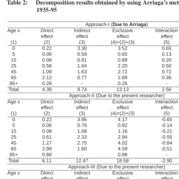
The results obtained by applying these formulae to the data under consideration are depicted in Table 2 as Approach-I (due to Arriaga, 1984).
Arriaga (1984:87) said that ‘both direct and indirect effects are generated because mortality has changed only within the age group under study’ (the assumption is that mortality has not changed in other age groups). If you recall, Chandra Sekar too defined ‘main effect’ in exactly the same fashion. So if one were to compare the results presented in Table 2 with Table 1 it is obvious that both effects are one and the same. A further com-parison reveals that Arriaga’s total effect (i.e., exclusive effect + interaction effect) yields exactly the same result as Chandra Sekar’s ‘Effect-interaction forwarded.’ In his later study Chandrasekaran (1986:7) mentions that ‘the difference between the expectation of life at birth recorded by the life tables (viz., 15.68) and the sum of all the main effects (viz., 13.13) is the sum of the interaction of all orders (viz., 2.55)’ reflecting once again the conclusion obtained in Approach-I of Arriaga. Having found this vital and interesting connection between the two methodologies I shall now attempt to extend the Arriaga’s method. These are represented as Approach-II and Approach-III. The formulae used in deriving the results presented in Table 2 are given below:
Arriaga’s Approach-II: Direct effect =i
DE x= l 2 x (e 2 x e 1 x
)+l 2 x (l 1 x+n e 1 x+n ) l 1 x (l 2 x+n e 2 x+n ) l 2 x (2.8)
Indirect effect =i IE x= e 2 x+n l 2 x+n l 2 x l 1 x+n l 1 x (2.9)
Table 2: Decomposition results obtained by using Arriaga’s method: US, females, 1935-95
Approach-I (Due to Arriaga)
Age x Direct Indirect Exclusive Interaction Total
effect effect effect effect effect
(1) (2) (3) (4)=(2)+(3) (5) (6)=(4)+(5)
0 0.22 3.30 3.52 0.65 4.17
5 0.06 0.59 0.65 0.13 0.78
15 0.08 0.81 0.89 0.20 1.09
25 0.56 1.64 2.20 0.50 2.70
45 1.09 1.63 2.72 0.72 3.44
65 2.12 0.77 2.89 0.36 3.25
85+ 0.26 - 0.26 - 0.26
Total 4.39 8.74 13.13 2.56 15.69
Approach-II (Due to the present researcher)
Age x Direct Indirect Exclusive Interaction Total
effect effect effect effect effect
(1) (2) (3) (4)=(2)+(3) (5) (6)=(4)+(5)
0 0.22 3.95 4.17 -0.65 3.52
5 0.06 0.76 0.82 -0.14 0.68
15 0.08 1.08 1.16 -0.21 0.95
25 0.61 2.33 2.94 -0.55 2.39
45 1.27 2.75 4.02 -0.84 3.18
65 2.99 1.60 4.59 -0.51 4.08
85+ 0.88 - 0.88 - 0.88
Total 6.11 12.47 18.58 -2.90 15.68
Approach-III (Due to the present researcher)
Age x Direct Indirect Exclusive Interaction Total
effect effect effect effect effect
(1) (2) (3) (4)=(2)+(3) (5) (6)=(4)+(5)
0 0.22 3.63 3.85 0.00 3.85
5 0.06 0.67 0.73 -0.00 0.73
15 0.08 0.94 1.02 -0.01 1.01
25 0.58 1.99 2.57 -0.02 2.55
45 1.18 2.19 3.37 -0.06 3.31
65 2.55 1.18 3.73 -0.07 3.66
85+ 0.57 - 0.57 - 0.57
Total 5.24 10.60 15.84 -0.16 15.68
Interaction effect =i I
x=i OE x i IE x= (e 2 x+n e 1 x+n ) l 2 x l 1 x+n l 1 x l 2 x+n (2.11) Where,i OE x= e 1 x+n l 2 x+n l 2 x l 1 x+n l 1 x (2.12)
Total effect =i DE x + i IE x + i I x= l 2 x (e 2 x e 1 x ) l 2 x+n (e 2 x+n e 1 x+n ) (2.13)
The formula for the open-ended age group is as follows:
DE x+ =l 2 x (e 2 x e 1 x ) (2.14) Arriaga’s Approach-III: Direct effect =i
DE x= (e 2 x e 1 x )(l 2 x +l 1 x ) 2 + (l 2 x +l 1 x ) l 1 x+n e 1 x+n l 1 x l 2 x+n e 2 x+n l 2 x 2 (2.15)
Indirect effect =i IE x= e 2 x+n l 2 x+n l 2 x l 1 x+n l 1 x e 1 x+n l 1 x+n l 1 x l 2 x+n l 2 x 2 (2.16)
The exclusive effect =i DE x + i IE x= (e 2 x e 1 x )(l 2 x +l 1 x ) 2 (e 2 x+n e 1 x+n ) l 1 x l 2 x+n l 2 x + l 2 x l 1 x+n l 1 x 2 (2.17)
Interaction effect =i I
Total effect =i DE
x +
i IE
x +
i I
x= (e
2 x
e 1 x
)(l 2 x
+l 1 x ) 2
(e 2 x+n
e 1 x+n
)(l 2 x+n
+l 1 x+n
) 2
(2.20)
The formula for the open-ended age group is as follows:
(e 2 x
e 1 x
)(l 2 x
+l 1 x ) 2
(2.21)
Arriaga’s Approach-III is an attempt to combine the results of Approach-I and II. Earlier Murthy (1992) used this Approach-III to analyze the state wise mortality situation in India. Comparing Arriaga’s Approach-II results in Table 2 with that of Chandra Sekar’s Approach in Table 1 reveals that, while his ‘operative effect’ is the same as Arriaga’s ‘exclusive effect’, his ‘effect-interaction deferred’ too is the same as the ‘total effect’ of Arriaga. The difference between expectation of life at birth and the sum of all the exclusive effects of Arriaga’s Approach-II is the total of the interaction effects of all orders (See Table 2).
Analysis: Like Chandrasekaran (1986), Arriaga (1984) too overlooked the contri-butions of researchers like Chandra Sekar (1949), Lopez and Ruzicka (1977), Andreev (1982) and Pollard (1982) and thus could not anticipate an extension of his methodology in the manner carried out in this study by the present researcher.
Arriaga invented a new methodological approach using the temporary life expectancy concept originally suggested by him. Also, he suggested decomposing the exclusive effect of an age group into direct and indirect components. It turns out that he not only defined interaction effects in the same way as Chandra Sekar (1949), but also suggested a formula to derive it.
A closer look at Arriaga’s Approach-III results shows that unlike in Approach-I and II here the contribution of the interaction effect to the total difference in life expectancy at birth is quite negligible. Approach-III therefore appears more acceptable than the first two. Also column 6 of Approach-III gives exactly the same results as that of Chan-drasekaran’s Approach-II, Andreev (1982), Pressat (1985), Pollard (1982) and also United Nations (1985). Thus Arriaga’s Approach-III succeeds in decomposing the well known and oft used United Nations (1985) formulae of ‘total effect’ into ‘direct’, ‘indirect’, ‘ex-clusive’, and ‘interaction’ effects.
2.3 Lopez and Ruzicka’s (1977) method
expectancies at birth into two components i.e. the ’exclusive effect’ due to a particular age group and the ’interaction effect’ owing to different age groups.
The formulae suggested by Lopez and Ruzicka (1977) may be expressed as:
e 2 0 e 1 0 =4e 0 0 = k X
E(x;x+n)+ k X
I(x;x+n) (3.1)
Where,
k X
E(x;x+n)= l 2 x l 1 x l 1 x (e 2 x e 1 x ) l 1 x+n (e 2 x+n e 1 x+n ) (3.2) and k X
I(x;x+n)=(e 2 x+n e 1 x+n ) l 2 x l 1 x+n l 1 x l 2 x+n (3.3)
Following Arriaga, we may rewrite equation (3.1) as:
Total effect =
l 2 x (e 2 x e 1 x ) l 2 x+n (e 2 x+n e 1 x+n ) (3.1)
In the above equation, while the term
P k
E(x;x+n)refers to the ‘exclusive effect’
(say) that represents “the effects of mortality differentials between the two time periods within specified age intervals.” the term
P k
I(x;x+n)points to the ‘interaction effect’
and “summarizes the cumulative effect of mortality interactions between age groups.” Arriaga’s (1984) definitions for ‘direct’ and ‘indirect effects’, tally with Lopez and Ruzicka’s ‘exclusive effect’ given in formulae 3.2. This in turn can be decomposed and written in ‘direct’ and ‘indirect’ effect terms as:
Direct effect =
l 2 x l 1 x l 1 x (e 2 x e 1 x
)+l 1 x+n e 1 x+n l 2 x+n e 2 x+n or l 2 x (e 2 x e 1 x
)+l 2 x l 1 x+n e 1 x+n l 1 x l 2 x+n e 2 x+n l 2 x (3.4)
Indirect effect =
e 2 x+n l 2 x+n l 2 x l 1 x+n l 1 x (3.5)
Table 3: Decomposition results obtained by using Lopez and Ruzicka’s method: US, females, 1935-1995
Approach-I (Due to the present researcher)
Age x Direct Indirect Exclusive Interaction Total
effect effect effect effect effect
(1) (2) (3) (4)=(2)+(3) (5) (6)=(4)+(5)
0 0.22 3.30 3.52 0.65 4.17
5 0.06 0.59 0.65 0.13 0.78
15 0.08 0.81 0.89 0.20 1.09
25 0.55 1.64 2.19 0.50 2.69
45 1.09 1.63 2.72 0.72 3.44
65 2.12 0.77 2.89 0.37 3.26
85+ 0.26 - 0.26 - 0.26
Total 4.38 8.74 13.12 2.57 15.69
Approach-II (Due to Lopez and Ruzicka)
Age x Direct Indirect Exclusive Interaction Total
effect effect effect effect effect
(1) (2) (3) (4)=(2)+(3) (5) (6)=(4)+(5)
0 0.22 3.95 4.17 -0.65 3.52
5 0.07 0.76 0.83 -0.14 0.69
15 0.09 1.08 1.17 -0.21 0.96
25 0.60 2.33 2.93 -0.55 2.38
45 1.28 2.75 4.03 -0.84 3.19
65 2.98 1.60 4.58 -0.51 4.07
85+ 0.88 - 0.88 - 0.88
Total 6.12 12.47 18.59 -2.90 15.69
Approach-III (Due to the present researcher)
Age x Direct Indirect Exclusive Interaction Total
effect effect effect effect effect
(1) (2) (3) (4)=(2)+(3) (5) (6)=(4)+(5)
0 0.22 3.63 3.85 0.00 3.85
5 0.06 0.67 0.73 -0.00 0.73
15 0.08 0.94 1.02 -0.01 1.01
25 0.58 1.99 2.57 -0.02 2.55
45 1.18 2.19 3.37 -0.06 3.31
65 2.55 1.18 3.73 -0.07 3.66
85+ 0.57 - 0.57 - 0.57
Total 5.24 10.60 15.84 -0.16 15.68
A comparison of the results in Panel 2, Table 3 with Table 1 clearly shows that the results obtained through the Lopez and Ruzicka method are a replica of the ’operative effect’ (’exclusive effect’ here) and ’effect interaction-deferred’ (’total effects’ here) of the Chandra Sekar’s procedure. The difference is that Lopez and Ruzicka succeeded in providing final formulae for ’interaction effect’ whereas Chandrasekaran failed to do so. A comparison of the results in Panel 2, Table 3 with Arriaga’s results (Panel 2, Table 2) indicates that both methods give approximately the same results.
In short one may extend the technique suggested by Lopez and Ruzicka to obtain the same results as Chandra Sekar (1949) and Arriaga (1984). I suggest therefore that the method suggested by Lopez and Ruzicka (1977) be represented as Lopez and Ruzicka Approach-II. Given below are the extended methodology formulae for Lopez and Ruz-icka’s Approach-I and Approach-III (as suggested by the present researcher).
Lopez and Ruzicka - Approach-I:
e 2 0 e 1 0 =4e 0 0 = k X
E(x;x+n)+ k X
I(x;x+n) (3.6)
Where,
k X
E(x;x+n)= l 1 x l 2 x l 2 x (e 2 x e 1 x ) l 2 x+n (e 2 x+n e 1 x+n ) (3.7) k X
I(x;x+n)=(e 2 x+n e 1 x+n ) l 1 x l 2 x+n l 2 x l 1 x+n (3.8)
We may rewrite equation (3.6) as:
Total effect =
l 1 x (e 2 x e 1 x ) l 1 x+n (e 2 x+n e 1 x+n ) (3.6)
Here, the formulae for ‘direct’ and ‘indirect’ effect are as follow:
Direct effect =
l 1 x l 2 x l 2 x (e 2 x e 1 x ) l 2 x+n e 2 x+n +l 1 x+n e 1 x+n or l 1 x (e 2 x e 1 x
)+l 1 x l 1 x+n e 1 x+n l 1 x l 2 x+n e 2 x+n l 2 x (3.9)
Indirect effect =
Lopez and Ruzicka - Approach-III: e 2 0 e 1 0 =4e 0 0 = k X
E(x;x+n)+ k X
I(x;x+n) (3.11)
Where,
k X
E(x;x+n)= (e 2 x e 1 x )(l 2 x +l 1 x ) 2 (e 2 x+n e 1 x+n ) l 1 x l 2 x+n l 2 x + l 2 x l 1 x+n l 1 x 2 (3.12) k X
I(x;x+n)=(e 2 x+n e 1 x+n ) 0 B @ l 1 x l 2 x+n l 2 x + l 2 x l 1 x+n l 1 x 2 (l 2 x+n +l 1 x+n ) 2 1 C A (3.13)
We may rewrite equation (3.11) as:
Total effect =
(e 2 x e 1 x )(l 2 x +l 1 x ) 2 (e 2 x+n e 1 x+n )(l 2 x+n +l 1 x+n ) 2 (3.11)
The formula for the open-ended age group is:
(e 2 x e 1 x )(l 2 x +l 1 x ) 2 (3.11a)
Direct and indirect effect for Lopez and Ruzicka’s Approach-III can be written as: Direct effect =
(e 2 x e 1 x )(l 2 x +l 1 x ) 2 + (l 2 x +l 1 x ) l 1 x+n e 1 x+n l 1 x l 2 x+n e 2 x+n l 2 x 2 (3.14)
Indirect effect =
e 2 x+n l 2 x+n l 2 x l 1 x+n l 1 x e 1 x+n l 1 x+n l 1 x l 2 x+n l 2 x 2 (3.15)
Sekar. The difference between these two is the ‘interaction effect’. Approach-III results given in panel three of Table 3 gives exactly the same values as given in Table 1(a). Results obtained here are also seen to be exactly the same as given in Arriaga’s Approach I and III.
Analysis: Lopez and Ruzicka’s (1977) method is also founded on the basic concept of ‘number of years lived’ first forwarded by Chandra Sekar (1949) and thus gives exactly the same formula for what it terms the ‘exclusive effect’. It is possible that they might not have been aware of the earlier study and therefore coined their own terms rather than staying with ‘main effect’ and ‘effect-interaction forwarded’ from Chandra Sekar.
However, Lopez and Ruzicka’s method is perfectly defined and they also derived the ‘interaction effect’ using a simpler formula. Also, juxtaposing Approach-III with the United Nations (1985) method (see section 2.6 of this paper for details of the discussion of United Nations(1985)) shows that the latter is identical to the Lopez and Ruzicka pro-cedure of Approach-III. And finally, the results of this approach also tally with Andreev (1982) and Pressat (1985) as the formulae used by them are completely similar.
Interpreting Lopez and Ruzicka’s results shows that all the points made by Chandra Sekar (1949) (as already discussed earlier as point 1 to 5) are valid; to these I propose to add another point (6) that, quite surprisingly, seems to have eluded Chandra Sekar (1949) in his classic study.
Point 6: The difference between the expectation of life at birth as recorded in the life tables, and the sum of all the operative effects, as in Chandra Sekar (1949) (‘exclusive effect’ in Approach-II of Lopez and Ruzicka and Approach-II of Arriaga), is the sum of the interaction of all orders.
2.4 Pollard’s (1982) method
Unlike other researchers, Pollard approached the problem by continuous analysis and used the ‘force of mortality’ concept. Pollard (1982:228) gave the following exact formula to measure changes in expectation of life at birth in terms of the effect these changes would have on different age groups:
(e 2 0
e 1 0
)= Z
1
0 (
1 x
2 x
)w x
dx (4.1)
Where, the weightw
xcan be obtained as:
w x
= 1 2 (
x p
1 0 e
2 x
+ x
p 2 0 e
1 x
And 1 x
and 2 x
are the forces of mortality at time 1 and 2 respectively.
The above formula combined ‘interaction’ with ‘main effect’ because ‘interaction terms are relatively small’. Further, it is ‘comparatively difficult to compute and not easy to interpret’. However, Pollard also defined interaction terms as ’effects arising from mortality changes in two or more age-groups.’ As the above formulae 4.1 is in integrals, and therefore difficult to use (not convenient for numerical purposes), Pollard (1982:229) provided another approximate formula (not given here) for the above formula (4.1) that can also be used for ’detecting and correcting minor errors’ in the expectation of life at birth.
About Pollard’s approach (using formula (4.1)) Chandrasekaran (1986:7) said that it ‘gives values for the different ages which is intermediate between the effect interaction deferred and effect-interaction forwarded’, thereby implying that Pollard’s results can also be compared well with the results obtained using Lopez and Ruzicka’s Approach-III, Arriaga’s Approach-III, and also the United Nations (1985) method.
Viewed critically, Pollard’s method demands detailed life tables for age groups ex-ceeding 85 years failing which it is difficult to measure the contribution made by the open-ended age group to the changes in life expectancy at birth. While he suggested sev-eral formulae in his various studies (see, Pollard, 1982, 1983 and 1988) for all practical purposes he showed a distinct preference for formula (4.1). Pollard’s (1988) also tried to compare his own method with Arriaga’s (1984). However when I compared Pollard’s (1982) technique with Arriaga’s (1984) and Lopez and Ruzicka’s (1977) I felt that had he transposed the formula he actually used with a different one for the comparison with Ar-riaga he might have got results that compared with ArAr-riaga’s Approach-1 and Lopez and Ruzicka’s Approach-1. I have provided here an extended version of Pollard’s approach that gives the same figures as obtained from methods discussed earlier in this study. Pol-lard’s approach is presented as Approach I, II and III. As PolPol-lard’s continuous approach is different from the discrete approaches presented here I have presented the extended versions in Appendix II.
2.5 United Nations (1982) method
The United Nations’ (1982:11) decomposition method given here is based on the general procedure suggested by Kitagawa (1955). The formulas may be rewritten here in life table terms ofl
xand e
xas given below:
4e 0
=(e 2 65
e 1 65
)
l 2 65
+l 1 65 2
(5.1)
The difference in life expectancy at birth attributable to mortality difference in those be-tween the ages of 30 and 65 can be obtained thus:
(e 2 30
e 1 30
)
l 2 30
+l 1 30 2
4e
0 (5.2)
And finally the difference in life expectancy at birth attributable to mortality differences in those below age 30 can be obtained thus:
(e 2 0
e 1 0
) (e 2 30
e 1 30
)
l 2 30
+l 1 30 2
(5.3)
Analysis: I quote from the United Nations (1982:11) study: “It should be noted that the decopositional procedure is not unique, since other formulas could be employed that would yield somewhat different results.” Perhaps the United Nations’ experience with the Lopez and Ruzicka (1977) method that gave the results shown in table IV.17 (United Na-tions, 1982:135) led them to conclude that different procedures might give varying results. Also, it would appear as if the United Nations was well aware of the other decomposition procedures of the time. On their procedure Chandrasekaran (1986:8) had this to say: “It dealt only with three age-groups and the extension of this approach to include more age groups becomes complicated.”
What is important is the fact that while the United Nations (1982) seemed to be aware of the existence of other decomposition formulas it failed to realize that all these proce-dures would give the same results if appropriate formulas were used. The fact that the 1985 study (detailed below) followed shows that there was an inclination to resolve this conundrum. To disprove Chandrasekaran’s (1986) statement and clarify that both United Nations 1982 and 1985 methods provide exactly the same result provided the identical age groups are considered in both the methods, I have shown in column 2(a) of Table 4 the outcome obtained if the age-groups are modified to 0-5, 5-15, 15-25, 25-45, 45-65, 65-85 and 85+. Thus both the United Nations 1982 and 1985 techniques now tally per-fectly.
Thus a general formula for the United Nations (1982) procedure may also be given as:
(e 2 x
e 1 x
)(l 2 x
+l 1 x ) 2
(e 2 x+n
e 1 x+n
)(l 2 x+n
+l 1 x+n
) 2
The formula does not cover the second term for the open-ended age group of 85 years and above; this can be worked out as:
(e 2 x
e 1 x
)(l 2 x
+l 1 x ) 2
(5.5)
Column 2 and 2(a) of Table 4 show the results of applying the above formula to the data of United States females 1935-1995.
Table 4: Decomposition results obtained using United Nations (1982) and United Nations (1985) methods: US, females,1935-1995
Age ’x’ United Nations (1982) Method United Nations
(2) Limited age (2a) More age (1985) Method
(1) groups groups (3)
0 6.24 (0-30 age group) 3.85 3.85
5 0.73 0.73
15 1.01 1.01
25 5.20 (30-65 age group) 2.54 2.54
45 3.32 3.32
65 3.66 3.66
85+ 4.24 (65+ age group) 0.57 0.57
Total 15.68 15.68 15.68
Source: Appendix Table 1
Unfortunately none of the United Nations publications elucidated that their 1982 and 1985 methodologies are the same, causing some confusion about the origin of the later technique. I hope to have dispelled this somewhat by clarifying that the second study is also the outcome of the decomposition method suggested by Kitagawa (1955), not Chan-drasekaran’s (1949) method or indeed any other decomposition procedure that followed or preceded that particular study.
2.6 United Nations (1985) method
The formula to find the contribution of the age groupx tox +n for a change ine 0 0
suggested by United Nations (1985) is as follows:
(e 2 x
e 1 x
)(l 2 x
+l 1 x ) 2
(e 2 x+n
e 1 x+n
)(l 2 x+n
+l 1 x+n
) 2
(6.1)
For the open-ended age group, United Nations suggested the following formula:
(e 2 x
e 1 x
)(l 2 x
+l 1 x ) 2
The above formula can be obtained from any of the methods (Approach-III of Ar-riaga’s method, Approach III of Lopez and Ruzicka’s method and the modified version of Chandrasekaran’s method) discussed in this study by merely adding the main effects to the interaction effects. This clearly gives the impression that United Nations probably derived its formula by using one of the above approaches or other formulae not elaborated upon here. As with Lopez and Ruzicka (1977), this formula was extensively used by the United Nations (United Nations, 1988) to study the contribution to sex differentials in life expectancy at birth of mortality differences within age group(x;x+n).
Analysis: As rightly stated by Chandrasekaran (1986:6), United Nations (1985) does not provide a basis or source for the derivation of formulae 6.1 and 6.2. While Chan-drasakaran (1986:8) has suggested that his procedure “helps to understand the implication of the United Nations (1985) method,” the present paper clearly shows that the basis of that study might well be the Lopez and Ruzicka Approach-III as well as any other method. On the other hand Shkolnikov et al., (2001:35) also conjecture that United Nations has used a simplified version of the formulae suggested by Andreev (1982) and Pressat (1985). The result of applying this formula to the data under consideration is provided in column 3, Table 4.
Unlike Chandrasekaran’s, Arriaga’s or Lopez and Ruzicka’s method, the United Na-tions method (United NaNa-tions, 1985) does not provide direct, indirect and other effects but is definitely the simplest, most intuitive and comprehensible method. I would therefore recommend that the United Nations’ (1985) technique be used for decomposition of total effect (or the difference between two life expectancies at birth) as a contribution from different age groups. However, in order to understand better the direct, indirect effects as defined by Arriaga (1984) I would suggest that Arriaga’s Approach III (in effect an extension of the United Nations’ 1985 method) is the better option. As a matter of fact Arriaga is the only researcher who attempted to split the ‘exclusive effect’ into ‘direct’ and ‘indirect’ components and suggest that they be considered individually. Thus one might use the ‘exclusive effect’ of Arriaga’s Approach-III when interested in studying only the total effect, exclusive of the total interaction effect. Similarly one might use only the ‘direct effect’ from the ‘exclusive effect’ if only interested in comprehending the effect of a particular age group on the total effect as has been done by Luy (2003).
3. Conclusions
are applied to a set of data. In order to prove my point I have extended the procedures suggested by Chandra Sekar (1949), Lopez and Ruzicka (1977), Arriaga (1984), Pollard (1982) and also the United Nations (1982). A new set of formulae has instead been pre-sented. Thus the Chandra Sekar (1949) method in its modified form along with Arriaga’s Approach-III, Lopez and Ruzicka’s Approach III, and United Nations (1982) method are seen to give same results as United Nations (1985), Pollard (1982), Andreev (1982), Pres-sat (1985). I have arrived at the conclusion that only the symmetric formulae of the above methods should be used in further studies on the subject because the percentage contri-bution of the sum of interaction terms to the difference in the life expectancy at birth is negligible.
4. Acknowledgements
This is a revised version of a paper earlier presented by me at the Poster Session of the Population Association of America 2003 Annual Meeting Program held at Minneapolis, Minnesota, May 1-3, 2003, Hilton Minneapolis and Towers. My sincere thanks to the PAA and funding agencies for making my trip possible. At the time of preparing this paper I was working as an Associate Professor at the Demographic Training and Research Center, Addis Ababa University, Addis Ababa, Ethiopia. I gratefully acknowledge Dr. Assefa Hailemariam, Associate Professor and Programme Coordinator of DTRC, AAU, AA, Ethiopia for his constructive comments and also for kindly permitting me to attend the conference.
References
Andreev, E.M. (1982). Method komponent v analize prodoljitelnosty zjizni. [the method of components in the analysis of length of life]. Vestnik Statistiki, 9, 42-47.
Andreev E.M., Shkolnikov V.M., Begun A.Z. (2002). Algorithm for decomposition of differences between aggregate demographic measures and its application to life expectancies, healthy life expectancies, parity-progression ratios and total fertility rates. Demographic Research, 7. (Article 14, Published 1 October 2002, Available at: www.demographic-research.org)
Arriaga, E.E. (1984). Measuring and explaining the change in life expectancies. Demog-raphy, 21, 83-96.
Canudas Romo, Vladimir. (2003). Decomposition methods in demography. Netherlands, Amsterdam: Rozenberg Publishers, Rozengracht 176A, 1016 NK.
Chandra Sekar, C. (1949). The effect of the change in mortality conditions in an age group on the expectation of life at birth. Human Biology, 21(1), 35-46.
Chandrasekaran, C. (1986). Assessing the effect of mortality change in an age group on the expectation of life at birth. Janasamkhya, 4(1), 1-9.
Das Gupta, Prithwis. (1993). Standardization and decomposition of rates: A user’s manual. U.S. Bureau of the Census, Current Population Reports, Washington, D.C., U.S. Government Printing Office, 23-186.
Kitagawa, E.M. (1955). Components of difference between two rates. Journal of the American Statistical Association, 50, 1168-1194.
Lopez, A.D. and Ruzicka, L.T. . (1977). The differential mortality of the sexes in aus-trialia. in n.d.mc glashan, (ed.) studies in australian mortality, tasmania: University of tasmania, environmental studies, occasional paper no.4 pollard, j.h. (1982) the expectation of life and its relationship to mortality. Journal of the Institute of Actu-aries, 109, Part 2(442), 225-240.
Luy, Marc . (2003). Causes of male excess mortality: Insights from cloistered popula-tions. Population and Development Review, 29(4), 647-676.
Murthy, P.K. and A.R. Gandhi. (2004). A revision of chandra sekar’s decomposition method and its application to sex differentials in mortality in india. Paper accepted for the poster session presentation of IUSSP XXV International Population Confer-ence to be held at Tours, France, 18-23 July 2005.
Pollard, J.H. (1982). The expectation of life and its relationship to mortality. The Journal of the Institute of Actuaries, 109, Part 2(442), 225-240.
Pollard, J.H. (1983). Some methodological issues in the measurement of sex mortality patterns. in Lopez, A.L. and L.T. Ruzicka (eds.) sex differentials in mortality: trends, determinants and consequences. Canberra: Australian National University.
Pollard, J.H. (1988). On the decomposition of changes in expectation of life and differ-entials in life expectancy. Demography, 25(2), 265-276.
Pressat. (1985). Contribution des ecarts de mortalite par age a la difference des vies moyennes. [the significance of variations in mortality by age on differences in life expectancy]. Population, 4-5, 765-70.
Preston, S.H., P.Heuveline and M.Guillot. (2001). Demography: Measuring and Mod-eling Population Processes, 65.
Pullum Thomas W., and JooEan Tan. (1992). Partitioning sources of change in the expec-tation of life. Paper presented at the Annual Meeting of the Population Association of America, Denver, Colorado, April 30 - May 2 1992.
Retherford, R.D. (1972). Tobacco smoking and the sex mortality differential. Demogra-phy, 9(2), 203-216.
Shkolnikov V.M., Andreev E.M., Begun A.Z. (2001). Gini coefficient as a life table function: computation from discrete data, decomposition of differences and empirical examples. MPIDR Working Paper, WP-2001-017. (Available at www.demogr.mpg.de)
United Nations. (1982). Levels and trends of mortality since 1950. ST/ESA/Ser. A/74. New York: United Nations, Department of International Economic and Social Af-fairs, Pp.11.
Eco-nomic and Social Affairs, 193.
United Nations. (1988). Sex differentials in life expectancy and mortality in devel-oped countries, an analysis by age groups and causes of death from recent and historical data. Population Bulletin of the United Nations, 65-107. (No.25-1988, ST/ESA/Ser.N/25. New York: United Nations, Department of International Eco-nomic and Social Affairs)
Appendix I
Appendix Table 1: Life table values for United States, Females, 1935 and 1995
Age ’x’ US, females, 1935 US, females, 1995
nm 1 x
l 1 x
e 1 x
nm 2 x
l 2 x
e 2 x
0 .047139 1.00000 63.32 .006830 1.00000 79.00
1 .004157 .95458 65.32 .000358 .99321 78.54
5 .001525 .93887 62.39 .000167 .99179 74.65
10 .001208 .93174 57.85 .000196 .99096 69.71
15 .002022 .92613 53.19 .000459 .98999 64.78
20 .002944 .91681 48.70 .000503 .98772 59.92
25 .003562 .90341 44.38 .000647 .98524 55.06
30 .003980 .88746 40.14 .000892 .98206 50.23
35 .005003 .86997 35.89 .001266 .97769 45.45
40 .005927 .84847 31.74 .001765 .97152 40.72
45 .008310 .82368 27.61 .002612 .96298 36.06
50 .011638 .79012 23.67 .004171 .95048 31.49
55 .016309 .74539 19.94 .006575 .93085 27.10
60 .024373 .68688 16.41 .010387 .90071 22.92
65 .035823 .60779 13.21 .016349 .85504 19.00
70 .055769 .50757 10.31 .024504 .78775 15.40
75 .092454 .38276 7.82 .038841 .69655 12.07
80 .130808 .23930 6.03 .063900 .57275 9.12
85+ .222482 .12281 4.49 .151106 .41424 6.62
Note: Source: Bell, F.C., A.H. Wade and S.C.Goss, (1992), Life Tables for the United States Social Security Aria: 1900-2080. Baltimore, Maryland, US Social Security Administration Office of the Actuary, Actuarial Study No.107, [nmx, andexcolumns were calculated fromlx;nLxandTxcolumns given in: Preston, S.H., P.Heuveline and
Appendix II
Technical note concerning Pollard’s (1982) method:
Pollard’s Approach-I:
Exclusive effect = EE= Z 1 0 [ n m 1 x n m 2 x ][l 1 x e 1 x
]dx (4.3)
The contribution of a particular age group (x, x+n), using the formula 4.3, is calculated as follows: [ n m 1 x n m 2 x ] h ( n 2 )(l 1 x e 1 x +l 1 x+n e 1 x+n ) i (4.4)
The contribution of an open-ended age group (x+) is calculated as follows by applying formula 4.3: [m 1 x+ m 2 x+ ] l 1 x e 1 x m 2 x+ (4.5)
Interaction effect = IE=
Z 1 0 [ n m 1 x n m 2 x ][l 1 x (e 2 x e 1 x
)]dx (4.6)
Therefore, the total effect = exclusive effect + interaction effect =
Z 1 0 [ n m 1 x n m 2 x ][l 1 x e 2 x
]dx (4.7)
Pollard’s Approach-II:
Exclusive effect = EE= Z 1 0 [ n m 1 x n m 2 x ][l 2 x e 2 x
]dx (4.8)
The contribution for the open-ended age (x+) is calculated as follows using formula 4.8: [m 1 x+ m 2 x+ ] ( l 2 x e 2 x m 1 x+ (4.10)
Interaction effect = IE=
Z 1 0 [ n m 1 x n m 2 x ][l 2 x (e 1 x e 2 x
)]dx (4.11)
Therefore, the total effect = exclusive effect + interaction effect =
Z 1 0 [ n m 1 x n m 2 x ][l 2 x e 1 x
]dx (4.12)
Pollard’s Approach-III:
Exclusive effect = EE=
Z 1 0 [ n m 1 x n m 2 x ] ( 1 2 )(l 1 x e 1 x +l 2 x e 2 x ) dx (4.13)
The contribution for a particular age group (x, x+n) is obtained as follows with formula 4.13: [ n m 1 x n m 2 x ] ( n 2 ) (l 1 x e 1 x +l 1 x+n e 1 x+n ) 2 + (l 2 x e 2 x +l 2 x+n e 2 x+n ) 2 (4.14)
The contribution for the open-ended age (x+) is obtained as follows with formula 4.13:
[m 1 x+ m 2 x+ ] ( 1 2 ) l 2 x e 2 x m 1 x+ + l 1 x e 1 x m 2 x+ (4.15)
Interaction effect = IE=
Z 1 0 [ n m 1 x n m 2 x ] (e 2 x e 1 x )(l 1 x l 2 x ) 2 dx (4.16)
Therefore, the total effect = exclusive effect + interaction effect =
Appendix Table 2: Decomposition results obtained by using Pollard’s method: US, females, 1935-1995
APPROACH-I (Due to the present researcher)
Age ’x’ Exclusive effect Interaction effect Total effect
(1) (2) (3) (4) = (2) + (3)
0 3.45 0.75 4.20
5 0.64 0.13 0.77
15 0.88 0.21 1.09
25 2.13 0.57 2.70
45 2.53 0.92 3.45
65 2.22 1.11 3.33
85+ 0.26 - 0.26
Total 12.11 3.69 15.80
APPROACH-II (Due to the present researcher)
Age ’x’ Exclusive effect Interaction effect Total effect
(1) (2) (3) (4) = (2) + (3)
0 4.32 -0.77 3.55
5 0.82 -0.14 0.68
15 1.17 -0.22 0.95
25 3.04 -0.64 2.40
45 4.36 -1.17 3.19
65 6.15 -2.06 4.09
85+ 0.88 - 0.88
Total 20.74 -5.00 15.74
APPROACH-III (Due to the present researcher)
Age ’x’ Exclusive effect Interaction effect Total effect
(1) (2) (3) (4) = (2) + (3)
(Due to Pollard)
0 3.89 -0.01 3.88
5 0.73 0.00 0.73
15 1.03 -0.01 1.02
25 2.58 -0.04 2.54
45 3.44 -0.12 3.32
65 4.18 -0.47 3.71
85+ 0.57 - 0.57
Total 16.42 -0.65 15.77
Results obtained by applying Pollard’s approach (as given above) to the data on US females 1935-1995 are presented in Appendix Table 2.
Analysis: Appendix Table 2 clearly indicates that the total does not precisely add up to the difference in life expectancy at birth of the two time periods under consideration; this is because of the use of approximate formulae derived from the continuous approach. Secondly, Pollard’s results compare well with that of other discrete methods, be they Lopez and Ruzicka, Arriaga, Chandra Sekar or United Nations. For instance, in Pollard’s Approach-I ‘exclusive effect’ equals Chandra Sekar’s ‘main effect’ and the ‘total effect’ equals Chandra Sekar’s ‘effect interactions forwarded’.