Volume 13 - Article 25 | Pages 615–640

in the population sciences published by the Max Planck Institute for Demographic Research Konrad-Zuse Str. 1, D-18057 Rostock · GERMANY www.demographic-research.org

DEMOGRAPHIC RESEARCH

VOLUME 13, ARTICLE 25, PAGES 615-640

PUBLISHED 21 DECEMBER 2005

http://www.demographic-research.org/Volumes/Vol13/25/ DOI: 10.4054/DemRes.2005.13.25

Research Article

Mortality tempo versus removal

of causes of mortality:

opposite views leading to different

estimations of life expectancy

Hervé Le Bras

2 Decreasing mortality as a sign of delay in deaths 616

3 Decreasing mortality as a change in the causes of death 619

4 Removing one cause of death: deeper insights 620

5 A numerical example of the two methods 621

6 Which life table is the reference table? 625

7 Unifying the two views: the repartition function of the delays by age and duration

626

8 Which is the best model? A discussion of the two methods 628

Bibliography 632

Appendixes

A Deaths and survivors of age x in t after the removal of a mortality cause in t= 0

633

B Demonstrating the strong properties of the two methods 634

Mortality tempo versus removal of causes of mortality:

opposite views leading to different estimations of life expectancy

Hervé Le Bras 1

Abstract

We propose an alternative way of dealing with mortality tempo. Bongaarts and Feeney have developed a model that assumes a fixed delay postponing each death. Our model, however, assumes that changes take place with the removal of a given cause of mortality. Cross-sectional risks of mortality by age and expectations of life therefore are not biased, contrary to the model of the two authors. Treating the two approaches as two particular cases of a more general process, we demonstrate that these two particular cases are the only ones that have general properties: The only model enjoying a decomposable expression is the removal model and the only model enjoying the proportionality property is the fixed delay model.

1 _{Ecole des Hautes Etudes en Sciences Sociales (EHESS) and Institut National d’Etudes Démographiques (INED), Paris.}

1. Introduction

A change in the timing of events does not exert the same influence on cross-sectional mortality indexes (i.e. life expectancy) as it does on fertility (i.e. the total fertility rate). The total fertility rate measures an intensity that is sensitive to the changing pace as well as delays or advances in events. In a life table, by contrast, the intensity remains equal to one because death occurs only once and all die in the end. Can we thus assert that timing has no effect on mortality indexes? In two recent papers (2,3), John Bongaarts and Griffith Feeney have taken the opposite stance, showing that delays or advances in mortality modified cross-sectional life expectancy. They found that the delay observed led to an overestimation by 2.4 years in France and by 1.6 years in the US and Sweden.

Following a brief overview of the computations made by the two authors, we propose an alternative way of dealing with mortality changes ; using multiple decrement life-tables and removing different causes of death. In contrast to the delay model advocated by Bongaarts and Feeney, our model shows no discrepancy between cross-sectional and longitudinal indexes. We argue that our model is more general than that of the above authors and more at pace with the true nature of mortality processes, the latter of which cannot be compared with nuptial or fertility processes. In brief, delays are a causal factor in the field of fertility and a consequential one in the field of mortality.

2. Decreasing mortality as a sign of delay in deaths

mortality and to build a life table, we find an expectation of life that is higher than during the preceding and following years. This is an example of the discrepancy introduced between longitudinal and cross-sectional measures when delays occur.

The same discrepancy is found when the delay changes (increases) continually through time. Le t=0 be the beginning of the process. The delay ending in t will be called f(t), s(x,t) denotes the survival function at age x and time t, and will be called S(x) before t=0, instead of s(x,0). With these notations, we get:

s(x,t) = S (x+t-f(t) - t) = S(x-f(t)).

The deaths since time t-f(t) or age x-f(t) were not postponed by a delay greater than f(t). From this we deduce an expression of deaths d(x,t)dt between t and t+dt (and x and x+dx) and of the forces of mortality q(x,t) by dividing these deaths by the survivors at that time and age:

d(x,t)dt = d(x,t)dx = s(x,t) - s(x+dt, t+dt), = S(x-f(t)) – S(x + dt - f(t+dt)),

= S(x-f(t)) –S(x-f(t)) – (1-f’(t))S’(x-f(t))dt, d(x,t) = (1-f’(t)) D(x-f(t)).

Consequently:

q(x,t) = (1-f’(t))µ(x-f(t)), (1)

where µ (x) is the force of mortality at age x and initial time t=0.

A simple case is that of a linear evolution of the delay at rate α which means that f (t) = αt. It follows that:

d(x,t) = (1-α )D(x- αt). (2)

The same relationship holds for the forces of mortality. By integrating them, the relationship can be expressed in terms of survivors:

s(x,t) = (S(x-αt)) (1-α).

Cross-sectional life expectancy at time t, e(t) is:

e(t) =

0

ω

∫

0

ω

=

0

ω

∫

If the delay is stabilized just after t, then the longitudinal expectation of life E(t) will become

E(t) =

0

ω

∫

The more the computation of e(t) overestimates the gain in life expectancy, the more rapidly the delay increases. For example, in Table 1 we computed the discrepancy value of the most recent life table for France for different values of the rate of increase (the delays were taken into account at age 36 and over).

Table 1: Overestimation of life expectancy at various rates of increase of the delay

Annual rate of increase of the delay (%) Overestimation(discrepancy)

5 0.44

10 0.86 15 1.26 20 1.65 25 2.02

At the rate of 25% we find a value not far from the one found by Bongaarts and Feeney (2,4). This is due to the actual rate of increase in life expectancy in France, which is approximately a quarter of a percent each year.

The entire process, in mathematical terms, results in a change in the time scale but not in the age scale, thus it is not necessary to go into further detail on the equations. The change in the time scale can be compared to a twisting of the life-lines on the Lexis diagram by a continuous deformation. In t, the deaths occurring during a small interval

∆t can be written as: d(x-f(t))(1- ∂f(t)/ ∂t)∆t; the survivors, S(x-f(t)), and the life table corresponding to the forces computed by dividing the deaths by the survivors have the survivorship functions:

S(x,t) = S(x-f(t))β(t) , (4)

3. Decreasing mortality as a change in the causes of death

4. Removing one cause of death: deeper insights

The method of suppressing causes of death leads to a delay in death, but there are different forms of delay. In the case postulated by Bongaarts and Feeney (we will call it the delay method or model), the delay applies to all individuals and is independent of age. As to the suppressed cause of death (we will call it the removal method or model), the delay affects only those struck by the particular cause, and this depends strongly on age. More precisely, let (S, µ, D), (S1, µ1, D1), (S2, µ2, D2), respectively, be the life table

(survivors, forces of mortality, deaths), first before the change, second for the specified cause, and third after the removal of this cause. This results in two very simple relationships:

µ1(x)+ µ2(x) = µ(x (5a) and S(x)=S1(x) S2(x). (5b)

Let us describe in greater detail the different stages of the decline in mortality: before t=0, the population follows the first mortality pattern (S, µ, D). Since time t=0, amongst those µ(x)S(x) who are assumed to die, µ2(x)dx do so and µ1(x)dx are saved

and follow from this point the second pattern of mortality (S2, µ2, D2). Therefore they

have a probability density of k(u)= D2(x+u)/S2(x) of dying after delay u. This is in line

with the hypothesis of independence of the causes of mortality: After being cured, the probability of dying from another cause is the same as in the general population of the same age. From these remarks, we can compute the deaths d(x,t) at age x and time t by taking in t at age x the endpoint of all delays (including 0):

d(x,t) =

0

t

∫

S(x-u)µ1(x) D2(x)/S2(x-u) du + µ2(x)S(x). (6)

Similarly, the survivors s(x,t) are those who have survived any cause of mortality at age x and S(x) and those who were hit at a former time t-u by the cause of death that was removed and whose delays are superior to u:

s(x,t) = S(x) +

0

t

∫

t at any time after t=0 and they are the same as those of the actual longitudinal pattern of mortality after t=0.

A sudden change in mortality preceded and followed by complete stability is not very realistic. The method of introducing a sudden change was used here, and was in the paper by Bongaarts and Feeney as well, to introduce a change of delays through time and not only at a fixed point in time. The same generalization as in delay can be made for the removal of a cause of death. We can assume that this removal is made at intervals T/n in n stages, each accounting for 1/n of the force of mortality µ1 (x).

Because the life table corresponding to the removal of each successive change is immediately followed by the population, the result, applicable separately for each elementary stage, holds for the whole change and can be made continuous by increasing n to infinity. For the same reason, the change does not need to be regular but can follow any time path. It is not even necessary to use the same age pattern; the only requirement is to have the table at the end without the removed cause or causes (S2, µ2, D2).

5. A numerical example of the two methods

The preceding results are abstract ones. Let us be more concrete in comparing the two methods using the same example. We assume the law of mortality defined over five years with survivorship function (100, 60, 30, 10, 0, 0) at age (0, 1, 2, 3, 4, 5). First, let us assume that a delay by half a year is gained by some mean since the beginning of the process at t=0 (Bongaarts and Feeney call this mean a « survival pill ») that automatically expands life by six months. If the deaths are spread regularly over each age, then we observe at each age only half of the deaths of the preceding years during the year following t=0 (Table 2). Thereafter, the deaths will be as numerous as before but shifted to half a year later (under the assumption that the newborns also take the miracle pill). Table 2 can be extended indefinitely, but this is not necessary because the numerical values are stabilized as of the second year after the change in the number of deaths, as well as for the survivors and quotients. The total number of deaths is the same as the preceding year 0, but the expectation of life is extended by half a year.

Now, let us take the same life table as in Table 3, before (year -1) and after (year 1) the change, but suppose it results from a sudden change of pattern due to the removal of a cause of death at time t=0. For that cause, the quotients of mortality Q1 are such

that

1-Q2(x) = (1-Q1(x)) (1-Q(x)),

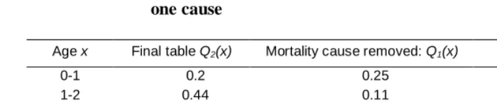
Table 2: Quotients of the life table before and after the removal of

one cause

Age x Final table Q2(x) Mortality cause removed: Q1(x) Initial table Q(x)

0-1 0.2 0.25 0.4

1-2 0.44 0.11 0.5

2-3 0.56 0.25 0.67

3-4 0.75 1.0 1.0

4-5 1.0

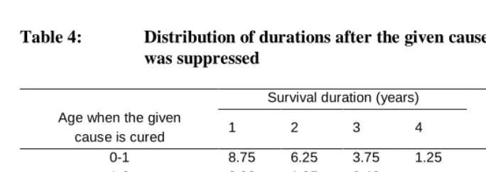
Each year following t=0, the survivors of the initial table are distributed in three groups: those who die from a cause of death in the final table, those who are facing death but survive, and those who will survive anyway. The second group dies according to the figures in the final table. For example, amongst the 40 foreseen deaths of the initial table at t=0, 20 die as given by the quotient of the final table, and the other 20 follow the pattern of the second table. Similarly, of the 30 individuals of the initial table who are prone to die within one or two years, 26.25 (30 x 0.44) die and 3.75 survive according to the figures in the final table. The survival times of those cured from the removed cause of death are distributed by duration, as shown in Table 4.

Table 3: An example of delay in mortality

Survivors and deaths Quotients

Time -1

Sur D

0

Sur D

1

Sur D

2

Sur D

3

Sur D

-1-0 0-1 1-2 2-3

Age

0 100 100 100 100 100

40 20 20 20 20 0.4 0.2 0.2 0.2

1 60 60 80 80 80

30 15 35 35 35 0.5 0.25 0.44 0.44

2 30 30 45 45 45

20 10 25 25 25 0.67 0.33 0.56 0.56

3 10 10 20 20 20

10 5 15 15 15 1.0 0.5 0.75 0.75

4 0 0 5 5 5

0 0 5 5 5 1.0 1.0

Deaths 100 50 100 100 100

(Total) Life ex-pectancy

Table 4: Distribution of durations after the given cause of death was suppressed

Survival duration (years)

Age when the given

cause is cured 1 2 3 4

Total surviving at the beginning 0-1 8.75 6.25 3.75 1.25 20

1-2 2.08 1.25 0.42 3.75

2-3 2.50 0.83 3.33

3-4 2.5 2.5

With this distribution, it is now possible to establish, at each successive year, the balance of deaths in the same way as in the preceding case of a given delay. We arrive at a similar table, in which the number of deaths is computed according to the delays ending in t at age x. For example, the 11.25 (7.5 + 2.5 + 1.25) dead during period 3-4 at age 3 in completed years come from 7.5 with delay 0 because they died from a cause other than the suppressed one, 2.5 with delay 1 from the preceding year and 1.25 with delay 2 coming from the preceding two years (see Table 4).

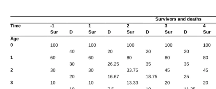
Table 5: An example of the removal of a mortality cause

Survivors and deaths Time -1

Sur D

1

Sur D

2

Sur D

3

Sur D

4

Sur D

5

Sur D

Age

0 100 100 100 100 100 100

40 20 20 20 20 20

1 60 60 80 80 80 80

30 26.25 35 35 35 35

2 30 30 33.75 45 45 45

20 16.67 18.75 25 25 25

3 10 10 13.33 20 20 20

10 7.5 10 11.25 15 15

4 0 0 2.5 3.33 5 5

0 0 2.5 3.33 3.755 5

Deaths

(Total) 100 70.42 86.25 94.58 98.75 100

Life expectancy 1.5 2.0 2.0 2.0 2.0 2.0

Quotients

Time -1-0 0-1 1-2 2-3

Age 0

0.4 0.2 0.2 0.2

1

0.5 0.25 0.44 0.44

2

0.67 0.33 0.56 0.56

3

1.0 0.5 0.75 0.75

4

1.0 1.0

6. Which life table is the reference table?

Bongaarts and Feeney contrast three ways of computing life expectancy: firstly, summing the survivors over the life course, secondly, taking the mean age at death in the standardized distribution of deaths, and thirdly, starting with the forces or quotients to construct the life table. In the real world, the last method is by far the most common one applied by statistical offices. The distributions of survivors or deaths are seldomly handled directly since they reflect generational history and are distorted by migrations. A cross-sectional life table is not intended to represent a remote past but to capture the actual trend. A usual justification of the cross-sectional life table, the fictitious generation, is that it can be observed in a generation for which all the observed data at time t are frozen and reproduced in the future during the time span of a generation.

This pseudo-empirical definition is not very useful. It seems better to freeze the causes that command the data rather than the data itself. With this causal approach, a good cross-sectional life table at time t is one that would be observed in a generation if suddenly all the parameters that configurate mortality were instantaneously immobilized at time t, including of course the advances and delays or the removal of some causes of mortality. In the preceding example where the two ways of change have been explored, the life table of reference is called the final life table. Its survivor and death functions emerged rapidly according to the delay method and progressively when a cause of mortality had been removed. However, with the removal method, the final table was immediately given by its quotients, in contrast to the delay method where fluctuations took place until the fixed delay was achieved. The issue, therefore, is not whether to choose between an estimation from the quotients, the survivors, or the deaths, but rather which life table constructed in the usual manner from the quotients provides an exact estimate of the longitudinal table corresponding to the « frozen » causes. Herein lies the large discrepancy between the model of delay and the model of removal.

Continuous change of causes through time is more problematic. In the removal model, the quotients of the longitudinal « frozen » table are immediately reached, owing to instantaneous adjustment. But with a change in delay f(t) through time t, the question arises: What is the behavior to be frozen at time t? Is it the behavior corresponding to the last (observed) delay ending just at t which began at t-f(t) and consequently, the behavior in t-f(t), or the behavior corresponding to the delay (non-observed) starting just in t ? The second solution is a more rational one, but the length of the delay beginning in t is unknown and will only be determined when it ends, by the mean age at the standardized deaths. The difference is not small, as the following example illustrates: if f(t) = αt (linear case), with t being the end point of the delay (see Appendix C), the delay beginning in t amounts to αt /(1-α). The difference d to delay

αt ending in t is quite high: d = αt /(1-α) -αt = α2t /(1-α). If the rate of increase is 25% and t = 30 (as in Europe), d = 2.5 years, and amusingly, equal to the overestimation computed by Bongaarts and Feeney. That is, there are no definite « frozen » causes in the delay model. Furthermore, there is naturally no empirical reference that can be used for building the hypothetical life-table during the process. If one needs to design a correction procedure, the reference must be defined prior to the correction, but this is not feasible in any circumstance.

7. Unifying the two views: the repartition function of the delays by

age and duration

The only difference between the two methods rests in the way by which the delays are postulated in formulating the two methods. We propose a more general model that covers the two instances considered so far. By the same token, we will demonstrate that they have strong and unique properties. Let us call λ(x-u,u) the density proportion of deaths foreseen to occur at age x-u and delayed at time t-u until age u is reached at time t, and let θ(x) be the proportion of deaths at age x non-delayed. By counting all delays which end in t at age x , we arrive at the number of deaths2:

d(x,t) =

0

t

∫

2 _{The formulae could be made simpler by working with Lebesgue measures instead of Riemann Integrals. All the terms would be put under the}

Using the same procedure, we recount the survivors as all those who have either never directly been threatened by death, or, if threatened, are cured and alive:

s(x,t) = S(x) +

0

t

∫

ω

∫

The two methods analyzed can be rewritten as follows:

for the removal method: λ(x,v) = (µ(x) - θ(x) ) D2(x+v) / S2(x).

θ(x) = µ2(x).

for the delay method: λ(x,v) = δ(v-T)µ(x),

where δ stands for the Dirac function and T for the fixed delay, θ(x) = 0.

Both methods have special properties. The removal method is the only decomposable method for which the forces of mortality by age adjust instantaneously to the final or longitudinal quotients of the table without the removed cause. The delay method assumes a fixed and common delay f(t) for every member of the population at any time t.

It is not a difficult but rather a tedious task to demonstrate the existence of these two properties. They are developed in Appendixes B and C. The first property is a good justification for using cross-sectional life expectancy as an indicator of longitudinal tendencies. It reveals, again, a large difference to fertility, where the total fertility rate is an inappropriate indicator of the evolution of the total number of children ever born.

The delay method is quite restrictive. Appendix C shows that it implies a common duration in the delay for all individuals. At time t-f(t), each death is delayed by f(t) exactly. This is not evident at first sight because the method starts from the proportionality rule. Nevertheless, it is a necessary consequence of the assumptions made. We can illustrate this with a simple model. In a single delay in t=0, assume that delay T applies only to a proportion p of the foreseen deaths at each age instead of being universal. The other 1-p deaths are in time according to the initial life-table. For t<T, the formulae (I) and (II) take the form:

d(x,t) = (1-p)µ(x) S(x) = (1-p)D(x),

s(x,t) = S(x) + p(S(x-t) - S(x)) = (1-p)S(x) + pS(x-t).

We see in the formula that the proportionality rule no longer exists, the denominator varying with age x. When delay T is over, the force of mortality becomes:

q(x,t) = ((1-p)D(x) + pD(x-T)) / ((1-p)S(x) + pS(x-T)).

The shift in the survivorship function is no longer constant, and depends on age because of the varying slope of S(x). The proportionality rule no longer applies. These remarks hold when the delay is not the same for all individuals but follows a probability distribution. A discussion of this issue is provided in Appendix C. The delay method is, therefore, restrictive. It supposes that at time t - f(t) every death without exception is postponed by a fixed duration f(t). From an empirical view, this seems unlikely. Below, we discuss the features and the likelihood of each method, delays or removal of the causes of death.

8. Which is the best model? A discussion of the two methods

The two models are now embedded in a common pattern of delays depending on age and time, yet the difference in the results is, so far, not suppressed. The delay model reveals an overestimation or an underestimation of life expectancy according to an increase or decrease in mortality. In the removal model, no overestimation, yet rather a correct estimation of the longitudinal trend, can be seen. Which method is the most appropriate one? Which model provides a more accurate representation of the process of changing mortality? The answers are found in the comparative handling of delays and risks. As its name indicates, the delay method moves the delays forward in time. The risks measured by the quotients and forces are the results of changing delays, which are the causal factor. The removal method, by contrast, sees the mortality change as a process of changing risks pertaining to certain causes. The delays are the consequence of changing risks through which the acting causes are channeled.

given period, one can rely on contraception and abortion in case of unwanted conception. The delays play a major role in fertility and nuptial processes because they involve the will. One can postpone the wedding day, even postpone it indefinitely, but one cannot do the same for the day of death, which is only partially influenced by our will.

There is another difficulty with the delay model. As demonstrated, all individual delays f(t) ending at time t are the same. Furthermore, they are postponed only once. If we enter the full details of the longitudinal process of mortality into the delay model, when a death is foreseen at age x, then the death is postponed until age x+f(t) but at that age, it becomes certain. There is no second chance of delay. It means that the population is split into two groups; those who are subject to a known date of death and those whose death has never been delayed. The expectations of life differ considerably in the two groups. In the removal model, by contrast, this difference disappears. After removing the given cause, all individuals run the same risk of death at a given age x. As mentioned before, the delays do not matter; they are the result of the process, not its cause. The new or final life-table is computed by changing the overall risks at each age in substracting the force of mortality of the given cause from the overall force of mortality. In the delay model, the new life-table is computed by the mean of the added delays. If we take a very long term view of mortality, say, from the Cro Magnon Era onwards, the process of mortality in the delay model results in the sum of many small delays of survival, each certain and the same for all individuals. This does not concur with the data on mortality. In such a model, there is no way to differentiate between individuals and no room for chance, and if it existed, then the resulting curve of deaths according to age should be Gaussian.

The removal model seems to be the more realistic one. In the long term, it depicts mortality as a process of removing the causes of mortality one after the other. To a demographer, this corresponds well with the analysis of mortality by cause and with the techniques of the multiple decrement life-table. In summation, mortality appears to be more of a multiplicative process than an additive one. One could say, nevertheless, that the language of delays and the language of causes of mortality are two different expressions of the same reality. This is not true, however. Knowing the delays T=f(t), we can compute the corresponding gain in risks at each age using the same notations as before:

µ2(x) = µ(x) - µ1(x) = µ(x - T). µ1(x) = µ(x) -µ(x-T).

If µ(x) follows the Gompertz law, µ(x) = Aerx, µ1(x) and µ2(x) also follow this law

µ1(x) = Aerx (1-e-rT ), µ2(x) = Aerx (e-rT ).

This property seems to be an empirical argument in favor of the delay method, because in the developed countries since the 1970s, the reduction of mortality has followed this pattern. Yet, as the preceding equations show, the same pattern can be generated with the removal of a cause of mortality displaying the same Gompertzian slope as the general mortality. Moreover, there is a one-to-one correspondence between delays and risks. In general, a given profile of risk by age has no equivalent in terms of delay. The removal method is more general. It allows for any risk profile, with µ1(x) < µ(x) being the only condition, whereas the delay method imposes a specific age profile of the risks.

In brief, the removal method is better suited to the process of mortality:

-Life expectancy after a postponed death is likely large, and not limited to a few months. However, if the delay is long, it provides a long duration with no risk of mortality. This is an unrealistic assumption, considering the nature of mortality.

-The delay is the same at any age in the delay method, yet it varies according to the expectation of life at age x in the removal method. This variation seems more realistic.

-The reference to the initial and final life tables is straightforward in the removal model, but not well defined during the course of the delay in the delay model.

-In the removal model, there is always one single population with every individual at age x who is threatened at any time by the same force of mortality, either µ(x) or

µ2(x). In the delay model, some individuals experiencing delay are exposed to high risks

and are near death, whereas the other individuals remain exposed to the usual risks. -The removal model is coherent with the analysis of mortality in terms of multiple decrements.

when they come to their end. The removal method does not raise such problems. At each point in time, the observed life table is the reference table.

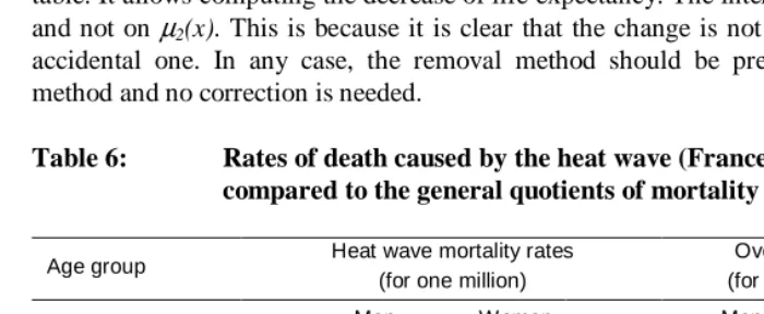
It does not follow from the discussion that any change of mortality pertains to the removal method. Only the long term changes or the trend in mortality obey such a model. In the short term, many causes of fluctuation are at work, suffice it to say seasonal variations related to atmospheric conditions, cold or hot weather, and influenza more severe than usual. They can delay or advance some deaths, but their effect is negligible on the average at a medium term range. The following statement could stem from Solomon: For the short term, take the delay method and for the long term, take the removal method. For short term fluctuations, the proportionality rule which is crucial for the working of the delay method, is not observed. Influenza, hot or cold weather, humidity or dry weather conditions, have a negative effect on very young and very old persons. A good example was provided by the heat wave that hit France in August 2003. The rates of mortality following the wave and computed for the age groups are reported in Table 6. Here, we can see how late and accelerated the increase of the probability of death was, and how far we are from proportionality when we compare these rates to the overall quotients at the same ages provided by the most recent French tables (2001).

The best way to tackle seasonal accidents remains the multiple decrement life table. It allows computing the decrease of life expectancy. The interest focuses on µ1(x)

and not on µ2(x). This is because it is clear that the change is not a permanent but an

accidental one. In any case, the removal method should be preferred to the delay method and no correction is needed.

Table 6: Rates of death caused by the heat wave (France, August 2003) compared to the general quotients of mortality

Age group Heat wave mortality rates (for one million)

Overall quotients (for one thousand) Men Women Men Women

60-64 115 050 65 27

65-69 244 138 99 41

70-74 396 281 149 69

75-79 786 673 226 122

80-84 1.901 1.923 356 227

85-89 2.759 2.821 528 400

90-94 5.702 6.696 712 620

Bibliography

Avdeev A., Blum A., Zakharov S., Andreev E.: The reaction of a heterogeneous population to perturbation, Population (Eng. sel). 10(2), 1998, 267-302.

Beaumel C., Doisneau L., Vatan M.: La situation démographique de la France en 2001, Paris, INSEE, 2003.

Bongaarts J., Feeney G.: How long we live, Population and Development Review, 28(1), 2002, 13-29.

Bongaarts J., Feeney G.: Estimating mean lifetime, PNAS, 2003.

Graunt J.: Natural and political observations..., London, John Martyn, 1661.

Le Bras H.: Simulation of change to validate demographic analysis, in Old and new methods in historical demography, Reher D., Schofield R. eds., 1993, 259-280.

Appendixes

A. Deaths and survivors of age x in t after the removal of a mortality cause in t= 0

The aim of the computation is to show that the force of mortality in t and x is independent of t and equal to its final value µ2(x). We have seen that the distribution of

delays u in t=0 at age x was u=0 in µ2(x) cases and f(u) = D2(x+u)/S2(x) in µ1(x) cases.

Conversely, the deaths at age x in t can be computed by adding up all the delays terminating in t at age x:

d(x,t) =

0

t

∫

= D2(x) 0

t

∫

because S(x) = S1(x) S2(x) et µ1(x-u) = - S1’ (x-u)/S1(x-u).

This results in: D2(x) = D2(x)

0

t

∫

= D2(x) (S1(x-t) -S1(x) ) + D2(x)S1(x) = D2(x)S1(x-t) if t < x

and = D2(x) (1 -S1(x) ) + D2(x)S1(x) = D2(x) if t > x.

We get the survivors s(x,t) at age x in t with the same kind of computation:

s(x,t) = S(x) +

0

t

∫

= S(x) +

0

t

∫

= S(x) +

0

t

∫

= S(x) + S2(x)

0

t

∫

= S(x)+ S2(x) (S1(x-t) -S1(x) ) = S2(x) S1(x-t) if t < x,

The mortality force q(x,t) = d(x,t)/s(x,t) follows:

q(x,t) = D2(x) S1(x-t) / S2(x) S1(x-t) = D2(x) / S2(x) = µ2(x) if t < x,

and = D2(x) / S2(x) = µ2(x) if t > x.

Therefore, for any t>0, the force of mortality at age x is the force of mortality µ2(x)

of the final life table (the initial table from which the given cause was removed under the assumption of independence).

B. Demonstrating the strong properties of the two methods

Let (S,D,µ) be the life table of reference, d(x,t) the density of deaths at age x in t >0, s(x,t) the survivors and λ(x-u,u) the probability for a death foreseen in t-u at age x-u to be delayed until age t (the delay is u). In summing all deaths in t at age x by considering the end of the delays and those who experience no delay, we get the same results as in Appendix A:

d(x,t) =

0

t

∫

s(x,t) = S(x) +

0

t

∫

ω

∫

A third relation results from the fact that the sum of the probability of the different situations for the foreseen death is the overall force of mortality µ (x):

0

ω

∫

As examples:

-λ(x,v) = ( µ(x) - θ(x) )D2(x+v) / S2(x),

when a cause of mortality is removed ((S2 , D2 , µ2 ) denotes the final life table).

-λ(x,v) = µ(x)f(v)

We will demonstrate that the removal method is the only decomposable method that keeps the force of mortality unchanged after t=0 and in this case gives θ(x) =

µ2(x).

Let use define: ϕ(x) = d(x,t) / s(x,t).

The derivative in t of the left part of this equation needs to be 0 for any t>0. Using the formulae (I) and (II), this can be written as:

∂d(x,t)/ ∂t.s(x,t) = d(x,t)∂s(x,t)/ ∂t.

S(x-t) λ(x-t,t)s(x,t) = d(x,t)S(t-x) ( t

ω

∫

so: λ(x-t,t)s(x,t) = d(x,t) ( t

ω

∫

t ω

∫

If we put the expression λ(x-t,t) in the formula (I) giving the deaths, we get:

d(x,t) = ϕ(x)

∫

t

S(x-u) ( u

ω

∫

according to (2)

= d(x,t) + S(x) (θ(x) - ϕ(x) ), thus:

ϕ(x) = θ(x), from what:

λ(x-t,t) = θ(x) ( t

ω

∫

Now take the decomposability assumption for λ(x-t,t):

Putting it in (4b), it becomes:

A(x-t)B(x) = θ(x) t

ω

∫

B(x) = θ(x) t

ω

∫

B(x) = θ(x) x

ω

∫

This formula is that of a life table, and more precisely, the final life table (S2, µ2,

D2), already encountered when looking at the removal of a cause of mortality.

Effectively:

B(x) = D2(x); S2(x) =

x ω

∫

ω

∫

There remains to determine the possible values for A(x-t). To that end, we need the equation (3):

0

ω

∫

0

ω

∫

A(x) x

ω

∫

A(x)S2(x) = µ(x) - µ2(x),

A(x) = (µ(x) - µ2(x)) / S2(x) .

we can now give the expression λ(x-t,t):

λ(x-t,t) = A(x-t)B(x),

= D2 (x)µ1 (x-t) / S2(x-t).

This is exactly the expression obtained when a cause of mortality described by the table (S1, µ1, D1) is removed in t=0. The method of removal, therefore, is the only

decomposable model for which the forces of mortality at any age x and any time t >0 catch up with their value in the actual longitudinal life table and does not depend on the time passed since the removal of the cause of mortality.

When the delays are independent of age, λ(x-t,t) can be written as:

λ(x-t,t) = µ(x-t)g(t).

Putting this expression in the equation (4b) for the equality of the cross-sectional and longitudinal life tables after the change in t=0, we get:

µ(x-t)g(t) = ϕ(x) ( t

ω

∫

g(t) = ϕ(x) t

ω

∫

It imposes ϕ(x) = k constant and g(t) = Ce –k.t.

Substituting in equations (I) and (II) for deaths d(x,t) and the survivors s(x,t), we arrive at a contradiction for their ratio that depends on t:

C. Fixed and variable delays

First, let us go back to the evaluation of deaths and forces of mortality from the value of the delays g(θ) taken at θ, the time of their beginning (and not f(t) taken at their end). Let θ be the time at the departure of the delay that ends at t. We get: t = θ + g(θ) = θ + f(t). Let us take a small interval ∆θ after θ. The delay beginning in θ + ∆θ will end in t1= θ + ∆θ + g(θ+ ∆θ) which is equivalent to θ + ∆θ + g(θ ) + g’(θ )∆θ. The interval ∆t between t and t1 is as follows:

∆t = (1 + g’(θ))∆θ.

At the end time in t, the density of delayed deaths is therefore at the ratio 1/(1 + g’(θ )) with the density of the deaths delayed at the departure between θ and θ + ∆θ. Consider now the increase of the delay at the point of arrival of the delay in t: between t and t1 , the delay f(t) grows by g’(θ )∆θ. Its derivative is:

f’(t) = g’(θ)∆θ / ∆t = g’(θ)∆θ / (1 + g’(θ)); ∆θ = g’(θ)/ (1 + g’(θ)).

This gives the formula for the deaths in case of delay:

d(x,t) = (1 – f’(t))D(x-f(t)) = 1 / (1 + g’(θ))D(x-g(θ)),

because 1 – f’(t) = 1- g’(θ)/ (1 + g’(θ)) = 1 / (1 + g’(θ)).

It is necessary to have the formula at the departure of the delay and not only at its arrival if we want to write the case where delay u varies according to the law of probability k(u)du. Let us demonstrate in these circumstances that the proportionality rule no longer holds. In consequence, the delay method necessarily rests on the particular hypothesis of a fixed delay. There is at a time t only one value for the delay for any individual threatened by death. We can begin the demonstration with the simple case of a sudden and unique change in t=0. The deaths at age x and time t will be:

d(x, t) =

Ξ ∞

∫

s(x, t) = S(x) +

0

t

∫

where:

K(u) = u

ω

∫

If the proportionality property holds, it is necessary that:

d(x,t) = p(t)D(x-l(t)). (8)

Integrating in the whole age range the two formulae of the deaths (6) and (8I) leads to:

0

t

∫

−∞

ω

∫

−∞

ω

∫

1-K(t) = p(t).

Under these conditions, we would get:

D(x-l(t)) =

0

t

∫

t

(k(u)/ (1-K(t)))D(x-u)du.

With (k(u)/ (1-K(t))) being a probability distribution on the interval of time {0,t}, the distribution of deaths should be at each age a weighted average of itself with a constant shift (playing the role of the delay). This is impossible a priori and a posteriori because the distributions of delays u, ( k(u)), and of deaths x, (D(x)), have no relationship.